K-modes & K-prototypes R代码

Author

Li Zongzhang

Published

October 17, 2025

Download icon 点击下载数据文件: supermarket.xlsx

加载必要的包

#install.packages("klaR")
library(klaR)
library(tidyverse)
library(readr)

导入数据并预处理

重命名
将定量变量转成factor
剔除含有缺失值的个案
将tibble转成data.frame

# 读取数据
library(readxl)
supermarket <- read_excel("supermarket.xlsx")

# 数据预处理
supermarket <- supermarket %>%
  rename(Marital = `Marital status`, Settlement = `Settlement size`) %>%
  mutate(
    Age_group = cut(Age, breaks = c(0,20,30,40,50,60,70,80), right = FALSE, 
                    labels = c("[0,20)","[20,30)", "[30,40)", "[40,50)", "[50,60)", "[60,70)", "[70,80)")),
    Income_group = cut(Income, breaks = c(0, 50000, 100000, 150000, 200000, 250000, 300000, 350000), 
                       right = FALSE, labels = c("[0,50k)", "[50k,100k)", "[100k,150k)", "[150k,200k)", 
                                                 "[200k,250k)", "[250k,300k)", "[300k,350k+)"))
  ) %>%
  select(Sex, Marital, Age_group, Education, Income_group, Occupation, Settlement) %>%
  mutate(across(.cols = everything(), .fns = as.factor)) %>%
  na.omit() %>% 
  as.data.frame()

重新命名因子水平

supermarket$Sex <- factor(supermarket$Sex, levels = c(0, 1), labels = c("Male", "Female"))
supermarket$Marital <- factor(supermarket$Marital, levels = c(0, 1), labels = c("Single", "Non-single"))
supermarket$Education <- factor(supermarket$Education, levels = c(0, 1, 2, 3), 
                                labels = c("Other/Unknown", "High School", "University", "Graduate School"))
supermarket$Occupation <- factor(supermarket$Occupation, levels = c(0, 1, 2), 
                                 labels = c("Unemployed/Unskilled", "Skilled Employee/Official", 
                                            "Management/Self-employed/Highly Qualified"))
supermarket$Settlement <- factor(supermarket$Settlement, levels = c(0, 1, 2), 
                                 labels = c("Small City", "Mid-sized City", "Big City"))

使用kmodes函数进行聚类分析

kmodes() 是一种基于随机初始化簇中心的聚类算法。

每次运行时，初始簇中心是随机选择的，所以可能得到不同的聚类结果。

使用 set.seed(123) 可以固定随机数生成器的状态，保证每次运行结果一致（可重复）。

set.seed(123)
kmodes_result <- kmodes(supermarket, modes = 4, iter.max = 10)

# 保存聚类结果
supermarket$Cluster <- as.factor(kmodes_result$cluster)

查看聚类结果

# 查看每个聚类的众数
kmodes_result$modes

     Sex    Marital Age_group   Education Income_group
1   Male     Single   [30,40) High School   [50k,100k)
2 Female Non-single   [20,30) High School  [100k,150k)
3 Female Non-single   [50,60)  University  [150k,200k)
4   Male     Single   [30,40) High School  [100k,150k)
                 Occupation     Settlement
1      Unemployed/Unskilled     Small City
2 Skilled Employee/Official     Small City
3 Skilled Employee/Official Mid-sized City
4 Skilled Employee/Official Mid-sized City

# 查看每个观测值的聚类分配
# kmodes_result$cluster
# 查看每个聚类的大小
kmodes_result$size

cluster
  1   2   3   4 
434 719 172 675

# 查看每个聚类的分布
table(supermarket$Cluster)


  1   2   3   4 
434 719 172 675

概括每个类别的特征

cluster_summary <- supermarket %>%
  group_by(Cluster) %>%
  summarise(
    Sex = names(which.max(table(Sex))),
    Marital = names(which.max(table(Marital))),
    Age_group = names(which.max(table(Age_group))),
    Education = names(which.max(table(Education))),
    Income_group = names(which.max(table(Income_group))),
    Occupation = names(which.max(table(Occupation))),
    Settlement = names(which.max(table(Settlement))),
    Size = n()
  )

# 输出簇特征
cluster_summary

# A tibble: 4 × 9
  Cluster Sex    Marital  Age_group Education Income_group Occupation Settlement
  <fct>   <chr>  <chr>    <chr>     <chr>     <chr>        <chr>      <chr>     
1 1       Male   Single   [30,40)   High Sch… [50k,100k)   Unemploye… Small City
2 2       Female Non-sin… [20,30)   High Sch… [100k,150k)  Skilled E… Small City
3 3       Female Non-sin… [50,60)   Universi… [150k,200k)  Skilled E… Mid-sized…
4 4       Male   Single   [30,40)   High Sch… [100k,150k)  Skilled E… Mid-sized…
# ℹ 1 more variable: Size <int>

可视化聚类结果

# 可视化：年龄组和收入组的簇分布
ggplot(supermarket, aes(x = Age_group, fill = Cluster)) +
  geom_bar(position = "dodge") +
  labs(title = "Age Group Distribution by Cluster", x = "Age Group", y = "Count") +
  theme_minimal() +
  theme(axis.text.x = element_text(angle = 45, hjust = 1))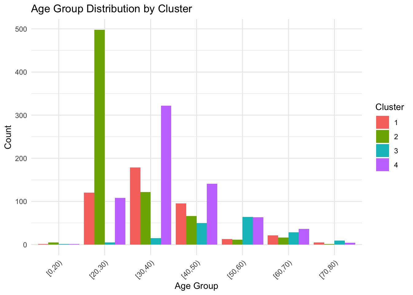

ggplot(supermarket, aes(x = Income_group, fill = Cluster)) +
  geom_bar(position = "dodge") +
  labs(title = "Income Group Distribution by Cluster", x = "Income Group", y = "Count") +
  theme_minimal() +
  theme(axis.text.x = element_text(angle = 45, hjust = 1))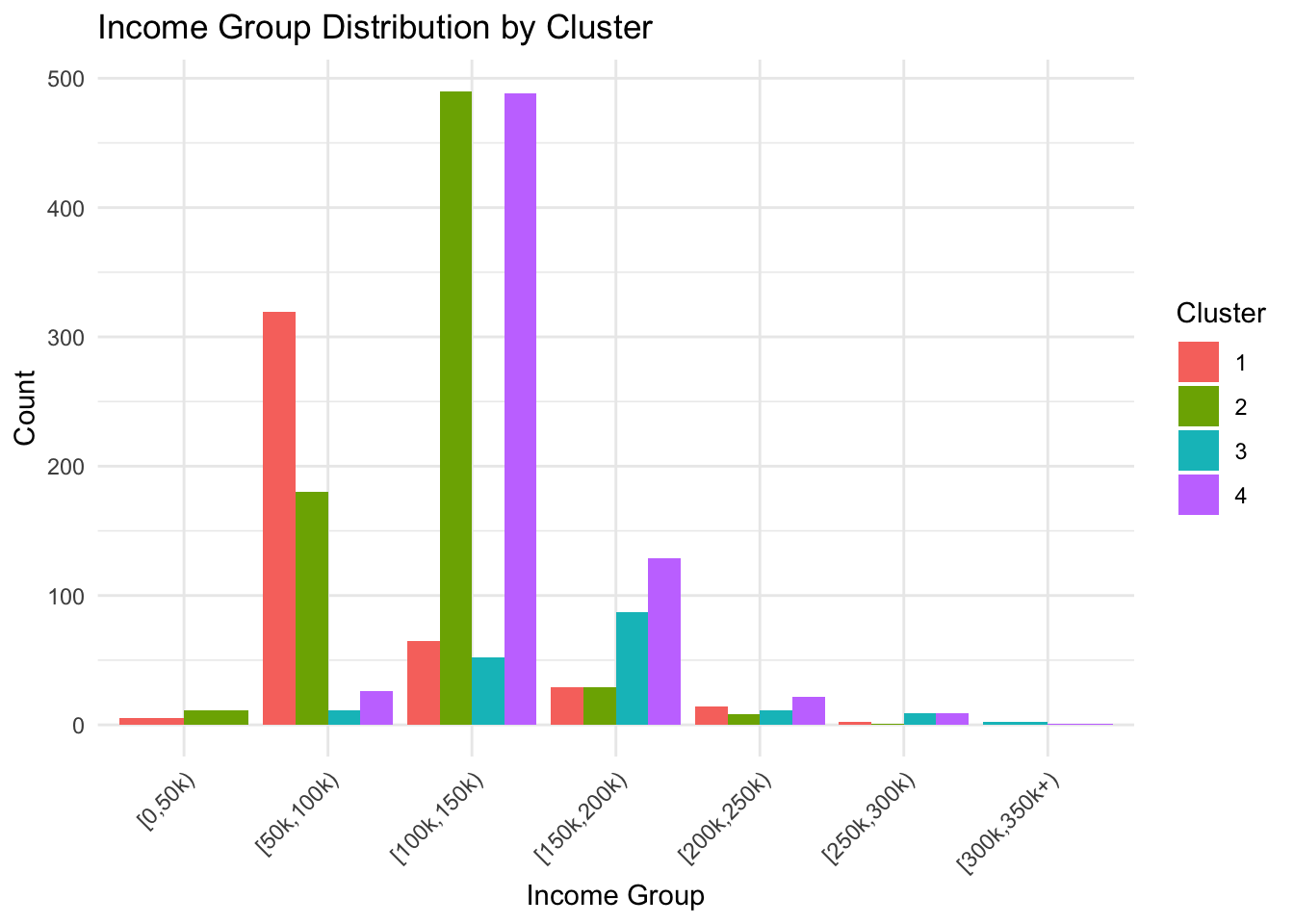

解释聚类结果

簇1：主要为年轻（[20,30)）、单身男性，高中教育，低收入（[0,50k)），失业/无技能，居住在小城市。
簇2：主要为中年（[30,40)）、已婚女性，大学教育，中等收入（[100k,150k)），熟练雇员，居住在中型城市。
簇3：主要为老年（[50,60)）、已婚混合性别，大学/研究生教育，高收入（[150k,200k)），高素质职业，居住在大城市。
簇4：可能为过渡群体，例如中年单身，高中/大学教育，中等收入，混合职业和居住地。

k-prototypes 聚类分析

# 指定图形的中文字体
par(family  = 'STKaiti')
#install.packages("showtext")
library(showtext)
showtext_auto()

library(clustMixType)

# 读取数据
supermarket <- read_csv("supermarket.csv")

# 数据预处理
# 读取数据
supermarket <- read_csv("supermarket.csv")

# 数据预处理
supermarket <- supermarket %>%
  rename(Marital = `Marital status`, Settlement = `Settlement size`) %>%
  select(Sex, Marital, Education, Occupation, Settlement, Income, Age) %>%
  mutate(across(c(Sex, Marital, Education, Occupation, Settlement), 
                as.factor)) %>%
  na.omit() %>% 
  as.data.frame()

# 设置随机种子
set.seed(123)

# 选择混合类型变量
mix_data <- supermarket %>%
  select(Age, Income, Sex, Marital, Education, Occupation, Settlement)

# 运行 k-prototypes 聚类，设定 4 个簇
kproto_result <- kproto(mix_data, k = 4, verbose = TRUE)

# NAs in variables:
       Age     Income        Sex    Marital  Education Occupation Settlement 
         0          0          0          0          0          0          0 
0 observation(s) with NAs.

Estimated lambda: 1357318162

# 查看聚类中心
kproto_result$centers

       Age   Income Sex Marital Education Occupation Settlement
1 31.69527 101157.4   1       1         1          1          0
2 43.93720 197277.5   0       1         1          2          1
3 36.19811 104039.5   0       0         1          1          0
4 39.33551 140742.7   0       0         1          1          2

# 每个样本的簇标签
head(kproto_result$cluster)

1 2 3 4 5 6 
4 4 3 4 4 4

# 各簇样本数量
table(kproto_result$cluster)


  1   2   3   4 
804 207 530 459

# 将簇标签添加到原始数据
supermarket$Cluster <- as.factor(kproto_result$cluster)


# 1️⃣ 数值变量在各簇的均值
num_summary <- supermarket %>%
  group_by(Cluster) %>%
  summarise(
    Mean_Age = mean(Age),
    Mean_Income = mean(Income),
    .groups = "drop"
  )
print(num_summary)

# A tibble: 4 × 3
  Cluster Mean_Age Mean_Income
  <fct>      <dbl>       <dbl>
1 1           31.7     101157.
2 2           43.9     197277.
3 3           36.2     104039.
4 4           39.3     140743.

# 2️⃣ 分类变量在各簇的分布
cat_vars <- c("Sex","Marital","Education","Occupation","Settlement")

cat_summary <- supermarket %>%
  group_by(Cluster) %>%
  summarise(across(all_of(cat_vars), ~paste(names(sort(table(.), decreasing = TRUE))[1])), 
            .groups = "drop")
print(cat_summary)

# A tibble: 4 × 6
  Cluster Sex   Marital Education Occupation Settlement
  <fct>   <chr> <chr>   <chr>     <chr>      <chr>     
1 1       1     1       1         1          0         
2 2       0     1       1         2          1         
3 3       0     0       1         1          0         
4 4       0     0       1         1          2

# 3️⃣ 可视化各簇样本数量
cluster_count <- supermarket %>%
  count(Cluster)

ggplot(cluster_count, aes(x = Cluster, y = n, fill = Cluster)) +
  geom_bar(stat = "identity") +
  labs(title = "各簇样本数量", x = "簇编号", y = "样本数量") +
  theme_minimal() +
  scale_fill_brewer(palette = "Set2")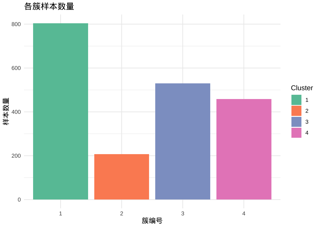

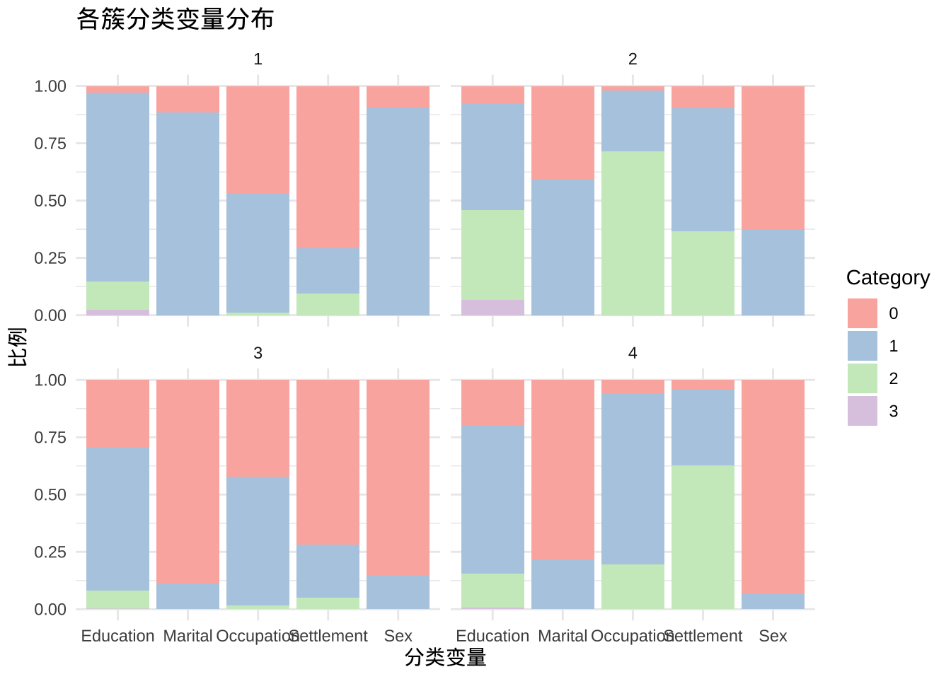
# 4️⃣ 可视化分类变量在各簇的分布（气泡图示例）
# 将分类变量展开
supermarket_long <- supermarket %>%
  pivot_longer(cols = all_of(cat_vars), names_to = "Variable", values_to = "Category")

ggplot(supermarket_long, aes(x = Variable, fill = Category)) +
  geom_bar(position = "fill") +
  facet_wrap(~Cluster) +
  labs(title = "各簇分类变量分布", y = "比例", x = "分类变量") +
  theme_minimal() +
  scale_fill_brewer(palette = "Pastel1")