十项全能运动员判别分析

Author

Li Zongzhang

Published

October 17, 2025

安装包

install.packages("ggplot2")
install.packages("tidyverse")
install.packages("MASS")
install.packages("klaR")
install.packages("devtools")
install.packages("psych")
install.packages("MVN")
install.packages("biotools")

加载包

library(ggplot2)
library(tidyverse)
library(psych)
library(biotools)
library(MVN)

数据文件

数据来源世界田联IAAF

Download icon 点击下载数据文件: decathlon.xlsx

导入数据

library(readxl)

decathlon <- read_excel("decathlon.xlsx", 
                        col_types = c("numeric", "text", "numeric", 
                                      "numeric", rep("text", 3), rep("numeric", 3), "text", 
                                      rep("numeric", 11)))

创建分类变量

library(tidyverse)
library(DescTools)
decathlon <- decathlon %>% mutate(tier = case_when(
  rank %[]% c(1,33) ~ "first",
  rank %[]% c(34,66) ~ "second",
  rank %[]% c(67,100) ~ "third",
  ))

多元正态检验

decathlon %>% 
  filter(tier == "first") %>%
  dplyr::select(M100:javelin_throw) %>%
  MVN::mardia()

             Test  Statistic    p.value     Method
1 Mardia Skewness 182.182632 0.97033157 asymptotic
2 Mardia Kurtosis  -1.844624 0.06509221 asymptotic

decathlon %>% 
  filter(tier == "second") %>%
  dplyr::select(M100:javelin_throw) %>%
  MVN::mardia()

             Test    Statistic    p.value     Method
1 Mardia Skewness 260.62023080 0.03144084 asymptotic
2 Mardia Kurtosis   0.03828022 0.96946426 asymptotic

decathlon %>% 
  filter(tier == "third") %>%
  dplyr::select(M100:javelin_throw) %>%
  MVN::mardia()

             Test   Statistic   p.value     Method
1 Mardia Skewness 226.3857853 0.3694740 asymptotic
2 Mardia Kurtosis  -0.2327665 0.8159428 asymptotic

检验协方差矩阵是否相等

df <- decathlon %>% 
  dplyr::select(M100:tier) %>% 
  mutate(tier = as.factor(tier)) %>% 
  as.data.frame()

boxM(df[, -11], df[, 11])


    Box's M-test for Homogeneity of Covariance Matrices

data:  df[, -11]
Chi-Sq (approx.) = 169.13, df = 110, p-value = 0.0002509

建立判别函数

library(MASS)
model <- lda(tier ~ M100 + Hurdles_M100 + M400 + M1500 +
             long_jump + high_jump + pole_vault +
             shot_put + discus_thow + javelin_throw, decathlon)
model

Call:
lda(tier ~ M100 + Hurdles_M100 + M400 + M1500 + long_jump + high_jump + 
    pole_vault + shot_put + discus_thow + javelin_throw, data = decathlon)

Prior probabilities of groups:
 first second  third 
  0.33   0.33   0.34 

Group means:
           M100 Hurdles_M100     M400    M1500 long_jump high_jump pole_vault
first  10.82909     14.51606 48.66818 277.9918  7.452424  2.006970   4.924242
second 11.05091     14.76273 49.88515 280.3267  7.202727  1.968182   4.668485
third  11.04735     14.72765 50.16412 278.9579  7.139706  1.946471   4.660882
       shot_put discus_thow javelin_throw
first  14.48636    44.79182      59.49242
second 13.97667    43.39879      58.46515
third  13.78294    41.44118      54.27412

Coefficients of linear discriminants:
                      LD1         LD2
M100           1.18999529 -0.42663574
Hurdles_M100   0.35551226 -0.88005615
M400           0.81924845  0.01025378
M1500          0.01210876 -0.01730195
long_jump     -1.76643422 -0.67067804
high_jump     -6.92011101 -1.04246407
pole_vault    -2.98252729  2.02264320
shot_put      -0.36594939  0.22228646
discus_thow   -0.18572931 -0.06791697
javelin_throw -0.07878029 -0.12571473

Proportion of trace:
   LD1    LD2 
0.9758 0.0242

预测样本中个案的类别

model.predict <- predict(model, decathlon)

decathlon$predict <- model.predict$class

评估预测效果

decathlon$ld1 <- model.predict$x[,1]
decathlon$ld2 <- model.predict$x[,2]

# 对比个案的观测类别的预测类别
table(decathlon$tier, decathlon$predict)

        
         first second third
  first     32      1     0
  second     0     30     3
  third      0      6    28

# 计算预测正确率
mean(decathlon$tier == decathlon$predict)

[1] 0.9

可视化

判别函数得分直方图

ldahist(model.predict$x[,1], model.predict$class)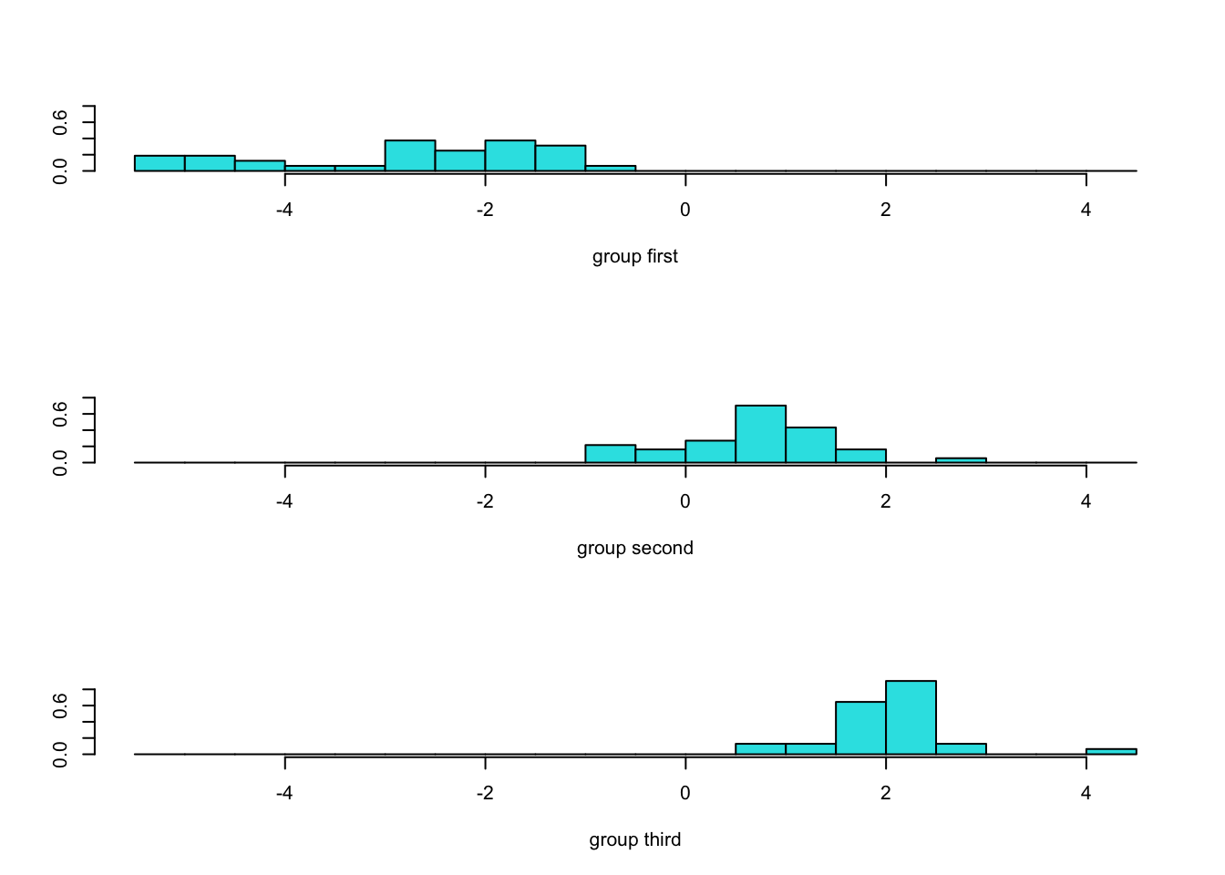

ldahist(model.predict$x[,2], model.predict$class)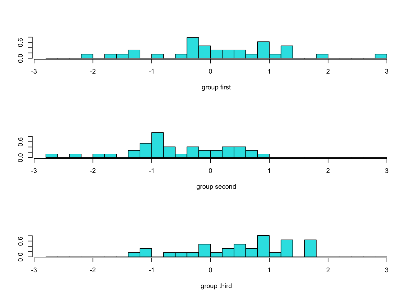

标记错误的个案

decathlon$right <- decathlon$tier == decathlon$predict


wrong_cases <- decathlon %>% 
  filter(decathlon$right == FALSE)

wrong_cases

# A tibble: 10 × 27
    rank COMPETITOR         `year of birth`   Age Nationality country  Continent
   <dbl> <chr>                        <dbl> <dbl> <chr>       <chr>    <chr>    
 1    32 Martin ROE                    1992    27 NOR         Norway   Europe   
 2    54 Akihiko NAKAMURA              1990    29 JPN         Japan    Asia     
 3    60 Ludovic BESSON                1998    21 FRA         France   Europe   
 4    65 Makenson GLETTY               1999    20 FRA         France   Europe   
 5    70 John LANE                     1989    30 GBR         United … Europe   
 6    71 Rik TAAM                      1997    22 NED         netherl… Europe   
 7    72 Nick GUERRANT                 1999    20 USA         United … North am…
 8    82 Kazuya KAWASAKI               1992    27 JPN         Japan    Asia     
 9    85 Elmo SAVOLA                   1995    24 FIN         Finland  Europe   
10    92 Aleksandar GRNOVIC            1996    23 SRB         Serbia   Europe   
# ℹ 20 more variables: Continent_code <dbl>, continent_G3 <dbl>,
#   continent_G4 <dbl>, VENUE <chr>, MARK <dbl>, M100 <dbl>,
#   Hurdles_M100 <dbl>, M400 <dbl>, M1500 <dbl>, long_jump <dbl>,
#   high_jump <dbl>, pole_vault <dbl>, shot_put <dbl>, discus_thow <dbl>,
#   javelin_throw <dbl>, tier <chr>, predict <fct>, ld1 <dbl>, ld2 <dbl>,
#   right <lgl>

decathlon %>% ggplot(aes(ld1, ld2, col = tier))+
  geom_point()+
  geom_point(data = wrong_cases,
             aes(ld1, ld2),
             col = "red", alpha = 0.6)+
  ylim(-5,5)+
  xlim(-5,5)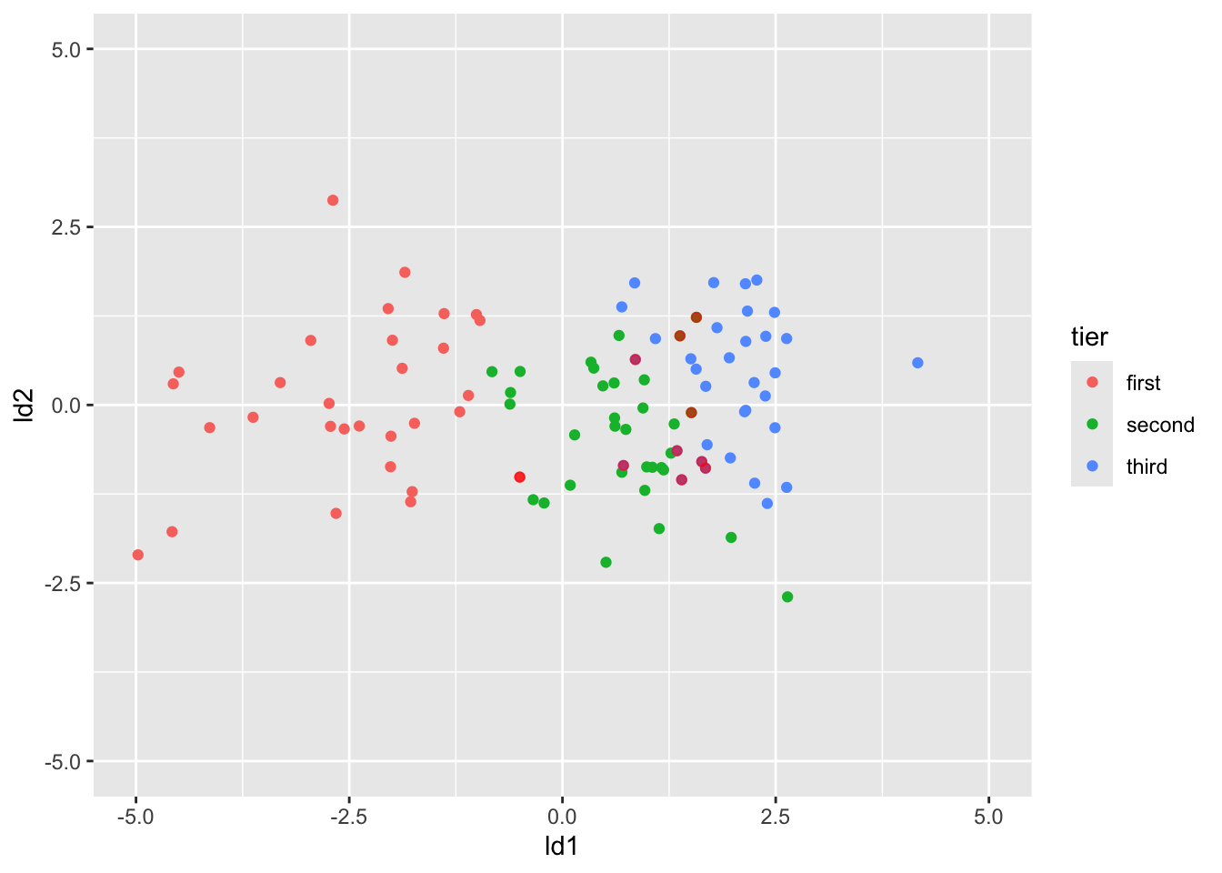

判别函数得分散点图，按类别着色

library(ggord)
ggord(model, decathlon$tier)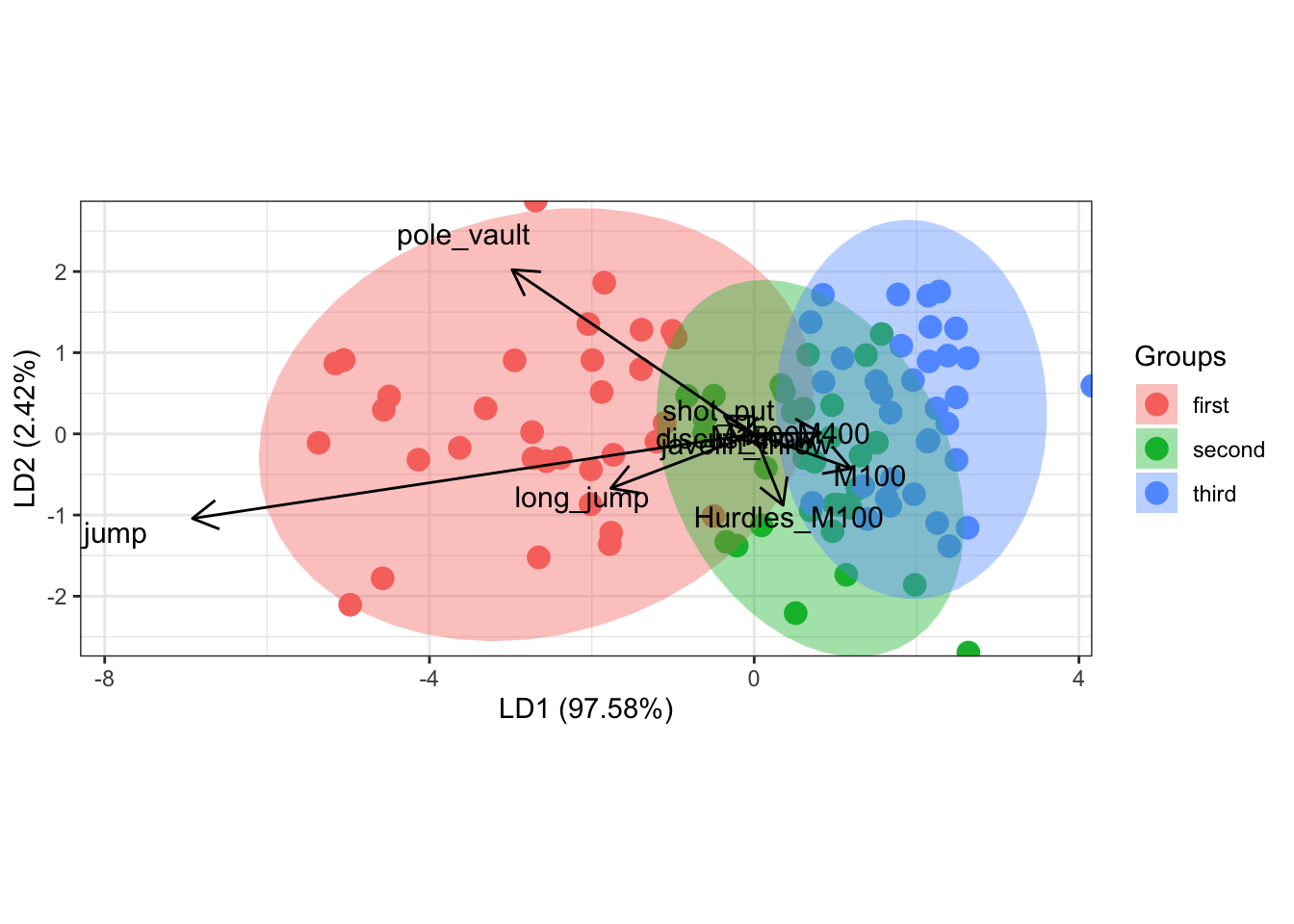

预测新个案

new_case <- data.frame(
  M100 = 10.73,
  Hurdles_M100 = 15.34,
  M400 = 47.93,
  M1500 = 288.58, 
  long_jump = 7.58, 
  high_jump = 2.06,
  pole_vault = 5.10,
  shot_put = 14.28,
  discus_thow = 36.93,
  javelin_throw = 61.43
  )

predict(model, new_case)

$class
[1] first
Levels: first second third

$posterior
      first      second        third
1 0.9967666 0.003214922 1.845589e-05

$x
        LD1        LD2
1 -2.719559 -0.3001785

new_pred <- predict(model, new_case)
new_scores <- new_pred$x # 提取LD1和LD2得分
new_class <- new_pred$class # 提取预测类别

在判别函数得分散点图中标记新个案

# 绘制基本ggord图
ggord(model, decathlon$tier) + 
  geom_point(data = data.frame(LD1 = new_scores[,1], 
                               LD2 = new_scores[,2], 
                               tier = new_class),
              aes(x = LD1, y = LD2),
              size = 5, shape = 17, color = "cyan") # 用大三角形标记新点