7 FA习题讲评

Author

Li Zongzhang

Published

October 23, 2025

教材P151 案例7.6

library(readr)
library(tidyverse)

case7_1 <- read_csv("case7.1.csv") %>% 
  rename(存货周转率 = x1, 
           总资产周转率 = x2, 
           流动资产周转率 = x3, 
           营业利润率 = x4, 
           毛利率 = x5, 
           成本费用利润率 = x6, 
           总资产报酬率 = x7, 
           净资产收益率 = x8, 
           每股收益率 = x9,
         扣除非经常性损益的每股收益 = x10,
         每股未分配利润 = x11,
         每股净资产 = x12
         )

# step 1
library(psych)
KMO(case7_1[-1])

Kaiser-Meyer-Olkin factor adequacy
Call: KMO(r = case7_1[-1])
Overall MSA =  0.79
MSA for each item = 
                存货周转率               总资产周转率 
                      0.82                       0.65 
            流动资产周转率                 营业利润率 
                      0.61                       0.80 
                    毛利率             成本费用利润率 
                      0.89                       0.77 
              总资产报酬率               净资产收益率 
                      0.77                       0.78 
                每股收益率 扣除非经常性损益的每股收益 
                      0.79                       0.79 
            每股未分配利润                 每股净资产 
                      0.89                       0.88

library(EFAtools)
BARTLETT(case7_1[-1])


✔ The Bartlett's test of sphericity was significant at an alpha level of .05.
  These data are probably suitable for factor analysis.

  𝜒²(66) = 1010.1, p < .001

# step 2

#计算特征值和特征向量
library(tidyverse)
case7_1.ev <- case7_1 %>% 
  select(-1) %>% cor() %>% 
  eigen()
case7_1.ev

eigen() decomposition
$values
 [1] 6.499533804 2.654940434 1.498015224 0.457112219 0.274204566 0.251019040
 [7] 0.107527371 0.097961610 0.067989899 0.055824591 0.026693650 0.009177591

$vectors
            [,1]         [,2]        [,3]         [,4]        [,5]
 [1,] 0.09244934 -0.477942255  0.05813051  0.841178011  0.03145094
 [2,] 0.14156255 -0.510840674 -0.24058789 -0.292348983 -0.01653565
 [3,] 0.11396951 -0.524423948 -0.24305043 -0.326001981 -0.23004977
 [4,] 0.31943729  0.092092805 -0.32649716  0.186801205 -0.46156889
 [5,] 0.26320084  0.359901186 -0.20646040  0.001269517 -0.12764452
 [6,] 0.33013418  0.251211794 -0.18956461  0.184085750 -0.15605637
 [7,] 0.34205073  0.132406992 -0.28087340 -0.013460429  0.30932073
 [8,] 0.34921919 -0.077629433 -0.27080622 -0.045567816  0.31120190
 [9,] 0.35203886 -0.016220410  0.33198939 -0.047641358  0.22911864
[10,] 0.35587756 -0.005797506  0.29858780 -0.035372439  0.21626107
[11,] 0.33113545 -0.098353749  0.32947303 -0.119334215  0.17254721
[12,] 0.28095737 -0.030775036  0.48410100 -0.108955477 -0.60873581
               [,6]        [,7]        [,8]        [,9]       [,10]       [,11]
 [1,] -0.1768332629  0.04573485 -0.03270303 -0.09875414  0.07971144 -0.01808396
 [2,] -0.2808558579 -0.14250773  0.07575002  0.57019837  0.29654994  0.23670175
 [3,] -0.0250653760  0.33986884 -0.12436745 -0.36834886 -0.39212881 -0.26817548
 [4,]  0.4907354140 -0.29243188 -0.17916257  0.25284266  0.04959833 -0.33165214
 [5,] -0.6623872468 -0.02297448 -0.49285071 -0.16465110  0.16926101 -0.05967790
 [6,]  0.0001332728  0.48738638  0.18625489  0.24484958 -0.39198754  0.49024948
 [7,] -0.0177809801  0.26740169  0.53232291 -0.12200012  0.37530228 -0.37541743
 [8,]  0.1836614909 -0.48270097  0.02303125 -0.46759327 -0.07678284  0.43511797
 [9,] -0.0676631801 -0.03966850  0.03201316  0.16744682 -0.18867682 -0.34464400
[10,] -0.1410113860 -0.24951050 -0.03736233  0.21446362 -0.43964946 -0.12369914
[11,]  0.3727798520  0.39358992 -0.48947667 -0.01017771  0.38644169  0.18250240
[12,] -0.1103111084 -0.12350439  0.37699725 -0.26605576  0.20542765  0.14203535
            [,12]
 [1,]  0.01452807
 [2,] -0.03681929
 [3,]  0.02732101
 [4,]  0.01088018
 [5,] -0.02772321
 [6,] -0.08684279
 [7,]  0.19712367
 [8,] -0.13649776
 [9,] -0.72196255
[10,]  0.63088779
[11,]  0.10907353
[12,]  0.02494923

#绘制碎石图
library(nFactors)

case7_1.ev$values %>% nScree() %>% 
  plotnScree(legend = F)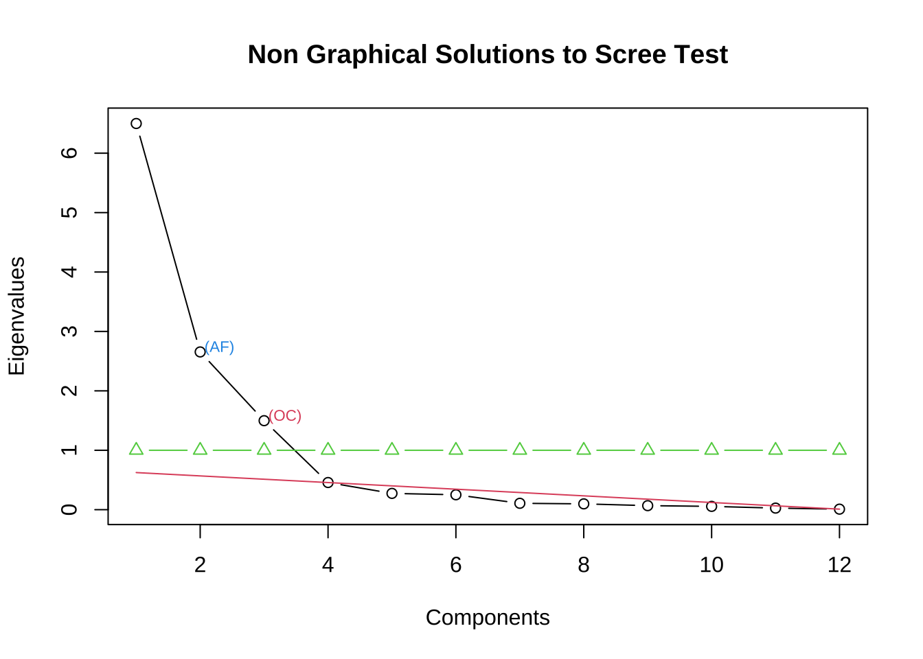

#未旋转
fa.pc.none <- principal(case7_1[-1], nfactors = 3,
                        rotate = "none")
fa.pc.none

Principal Components Analysis
Call: principal(r = case7_1[-1], nfactors = 3, rotate = "none")
Standardized loadings (pattern matrix) based upon correlation matrix
                            PC1   PC2   PC3   h2    u2 com
存货周转率                 0.24  0.78 -0.07 0.67 0.333 1.2
总资产周转率               0.36  0.83  0.29 0.91 0.090 1.6
流动资产周转率             0.29  0.85  0.30 0.90 0.097 1.5
营业利润率                 0.81 -0.15  0.40 0.85 0.155 1.5
毛利率                     0.67 -0.59  0.25 0.86 0.142 2.3
成本费用利润率             0.84 -0.41  0.23 0.93 0.070 1.6
总资产报酬率               0.87 -0.22  0.34 0.93 0.075 1.4
净资产收益率               0.89  0.13  0.33 0.92 0.081 1.3
每股收益率                 0.90  0.03 -0.41 0.97 0.029 1.4
扣除非经常性损益的每股收益 0.91  0.01 -0.37 0.96 0.043 1.3
每股未分配利润             0.84  0.16 -0.40 0.90 0.099 1.5
每股净资产                 0.72  0.05 -0.59 0.87 0.133 1.9

                       PC1  PC2  PC3
SS loadings           6.50 2.65 1.50
Proportion Var        0.54 0.22 0.12
Cumulative Var        0.54 0.76 0.89
Proportion Explained  0.61 0.25 0.14
Cumulative Proportion 0.61 0.86 1.00

Mean item complexity =  1.6
Test of the hypothesis that 3 components are sufficient.

The root mean square of the residuals (RMSR) is  0.03 
 with the empirical chi square  9.42  with prob <  1 

Fit based upon off diagonal values = 1

fa.pc.varimax <- principal(case7_1[-1], nfactors = 3,
                           rotate = "varimax")
fa.pc.varimax

Principal Components Analysis
Call: principal(r = case7_1[-1], nfactors = 3, rotate = "varimax")
Standardized loadings (pattern matrix) based upon correlation matrix
                             RC1  RC3   RC2   h2    u2 com
存货周转率                 -0.15 0.26  0.76 0.67 0.333 1.3
总资产周转率                0.13 0.07  0.94 0.91 0.090 1.1
流动资产周转率              0.08 0.02  0.95 0.90 0.097 1.0
营业利润率                  0.88 0.22  0.16 0.85 0.155 1.2
毛利率                      0.85 0.21 -0.32 0.86 0.142 1.4
成本费用利润率              0.89 0.35 -0.12 0.93 0.070 1.3
总资产报酬率                0.91 0.30  0.10 0.93 0.075 1.2
净资产收益率                0.79 0.34  0.42 0.92 0.081 1.9
每股收益率                  0.40 0.89  0.12 0.97 0.029 1.4
扣除非经常性损益的每股收益  0.43 0.87  0.12 0.96 0.043 1.5
每股未分配利润              0.31 0.87  0.23 0.90 0.099 1.4
每股净资产                  0.15 0.92  0.04 0.87 0.133 1.1

                       RC1  RC3  RC2
SS loadings           4.25 3.64 2.77
Proportion Var        0.35 0.30 0.23
Cumulative Var        0.35 0.66 0.89
Proportion Explained  0.40 0.34 0.26
Cumulative Proportion 0.40 0.74 1.00

Mean item complexity =  1.3
Test of the hypothesis that 3 components are sufficient.

The root mean square of the residuals (RMSR) is  0.03 
 with the empirical chi square  9.42  with prob <  1 

Fit based upon off diagonal values = 1

#按因子载荷系数降序排列
print(fa.pc.varimax$loadings, digits = 3, cutoff = 0.5,sort = T)


Loadings:
                           RC1    RC3    RC2   
营业利润率                  0.877              
毛利率                      0.845              
成本费用利润率              0.892              
总资产报酬率                0.910              
净资产收益率                0.792              
每股收益率                         0.894       
扣除非经常性损益的每股收益         0.869       
每股未分配利润                     0.866       
每股净资产                         0.918       
存货周转率                                0.758
总资产周转率                              0.942
流动资产周转率                            0.947

                 RC1   RC3   RC2
SS loadings    4.246 3.638 2.769
Proportion Var 0.354 0.303 0.231
Cumulative Var 0.354 0.657 0.888

#绘制因子载荷系数图
fa.diagram(fa.pc.varimax$loadings, digits = 3)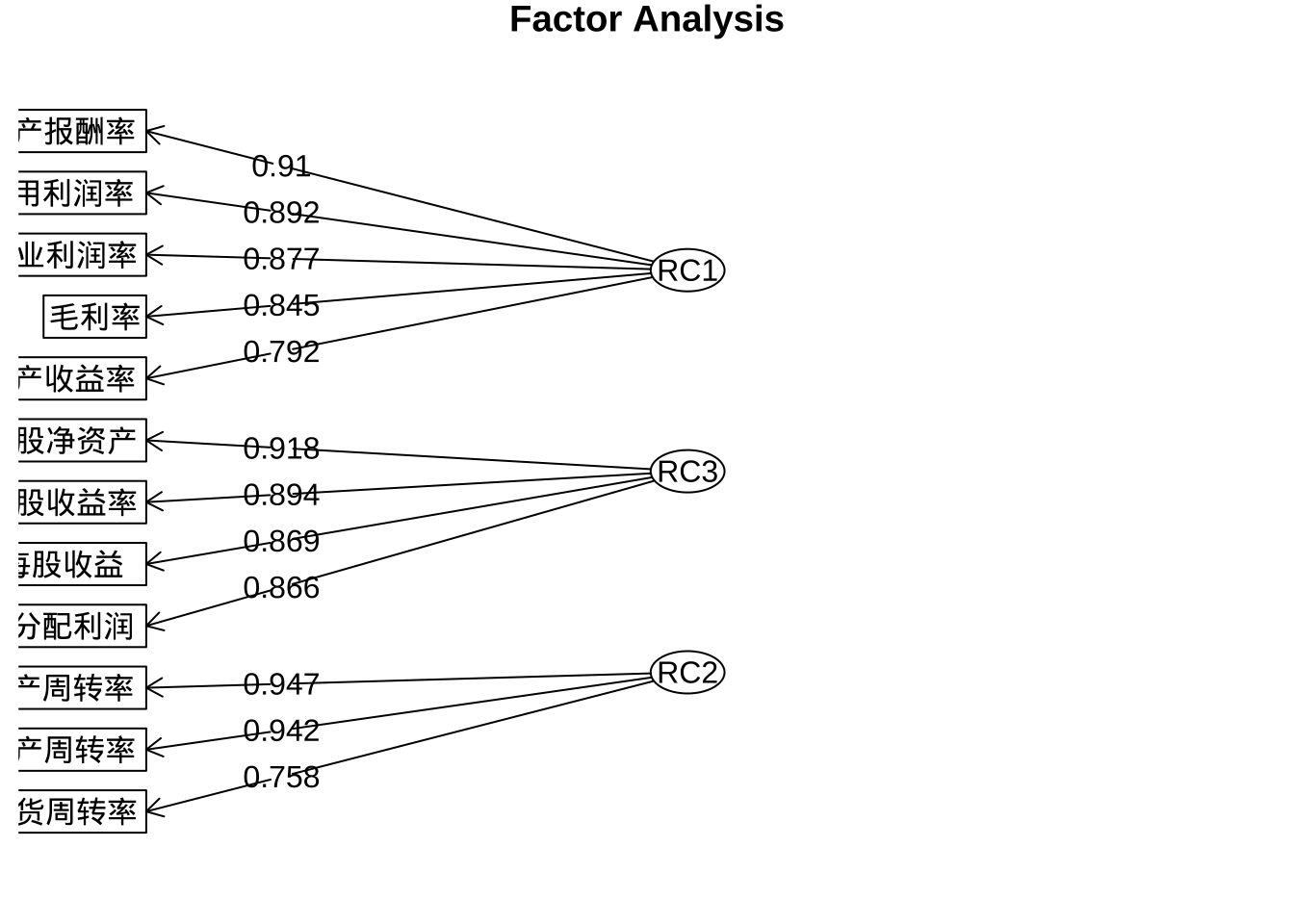

plot(fa.pc.varimax$loadings, type = "n")

library(psych)
fa.ml.varimax <- fa(case7_1[-1], 
                  nfactors = 3, 
                  fm = "ml",
                  rotate = "varimax")

fa.ml.varimax

Factor Analysis using method =  ml
Call: fa(r = case7_1[-1], nfactors = 3, rotate = "varimax", fm = "ml")
Standardized loadings (pattern matrix) based upon correlation matrix
                             ML3  ML1   ML2   h2     u2 com
存货周转率                 -0.11 0.23  0.63 0.46 0.5381 1.3
总资产周转率                0.11 0.09  0.95 0.92 0.0785 1.0
流动资产周转率              0.06 0.02  0.96 0.92 0.0803 1.0
营业利润率                  0.86 0.20  0.15 0.80 0.1957 1.2
毛利率                      0.81 0.22 -0.28 0.79 0.2126 1.4
成本费用利润率              0.89 0.34 -0.12 0.92 0.0768 1.3
总资产报酬率                0.90 0.32  0.10 0.92 0.0769 1.3
净资产收益率                0.77 0.36  0.41 0.90 0.1029 2.0
每股收益率                  0.39 0.91  0.12 1.00 0.0048 1.4
扣除非经常性损益的每股收益  0.42 0.88  0.12 0.98 0.0246 1.5
每股未分配利润              0.31 0.85  0.23 0.87 0.1311 1.4
每股净资产                  0.16 0.85  0.07 0.76 0.2448 1.1

                       ML3  ML1  ML2
SS loadings           4.09 3.55 2.59
Proportion Var        0.34 0.30 0.22
Cumulative Var        0.34 0.64 0.85
Proportion Explained  0.40 0.35 0.25
Cumulative Proportion 0.40 0.75 1.00

Mean item complexity =  1.3
Test of the hypothesis that 3 factors are sufficient.

df null model =  66  with the objective function =  18.65 with Chi Square =  1010.1
df of  the model are 33  and the objective function was  1.75 

The root mean square of the residuals (RMSR) is  0.02 
The df corrected root mean square of the residuals is  0.03 

The harmonic n.obs is  60 with the empirical chi square  4.1  with prob <  1 
The total n.obs was  60  with Likelihood Chi Square =  91.42  with prob <  2.2e-07 

Tucker Lewis Index of factoring reliability =  0.871
RMSEA index =  0.171  and the 90 % confidence intervals are  0.132 0.216
BIC =  -43.7
Fit based upon off diagonal values = 1
Measures of factor score adequacy             
                                                   ML3  ML1  ML2
Correlation of (regression) scores with factors   0.98 0.99 0.98
Multiple R square of scores with factors          0.96 0.99 0.96
Minimum correlation of possible factor scores     0.92 0.97 0.92

#按因子载荷系数降序排列
print(fa.ml.varimax$loadings, digits = 3, cutoff = 0.5,sort = T)


Loadings:
                           ML3    ML1    ML2   
营业利润率                  0.862              
毛利率                      0.812              
成本费用利润率              0.892              
总资产报酬率                0.901              
净资产收益率                0.771              
每股收益率                         0.911       
扣除非经常性损益的每股收益         0.884       
每股未分配利润                     0.847       
每股净资产                         0.851       
存货周转率                                0.628
总资产周转率                              0.949
流动资产周转率                            0.957

                 ML3   ML1   ML2
SS loadings    4.090 3.549 2.594
Proportion Var 0.341 0.296 0.216
Cumulative Var 0.341 0.637 0.853

#函数psych::fa，varimax旋转
library(psych)
fa.pa.varimax <- fa(case7_1[-1], 
                    nfactors = 3, 
                    fm = "pa",
                    rotate = "varimax")

print(fa.pa.varimax$loadings, digits = 3, cutoff = 0.5,sort = T)


Loadings:
                           PA1    PA3    PA2   
营业利润率                  0.839              
毛利率                      0.816              
成本费用利润率              0.896              
总资产报酬率                0.906              
净资产收益率                0.780              
每股收益率                         0.913       
扣除非经常性损益的每股收益         0.878       
每股未分配利润                     0.848       
每股净资产                         0.851       
存货周转率                                0.640
总资产周转率                              0.943
流动资产周转率                            0.944

                 PA1   PA3   PA2
SS loadings    4.094 3.533 2.594
Proportion Var 0.341 0.294 0.216
Cumulative Var 0.341 0.636 0.852

plot(fa.pc.varimax$loadings[,1], 
     fa.pc.varimax$loadings[,2])

text(fa.pc.varimax$loadings[,1], 
     fa.pc.varimax$loadings[,2], 
     rownames(fa.pc.varimax$loadings),
     cex = 0.3)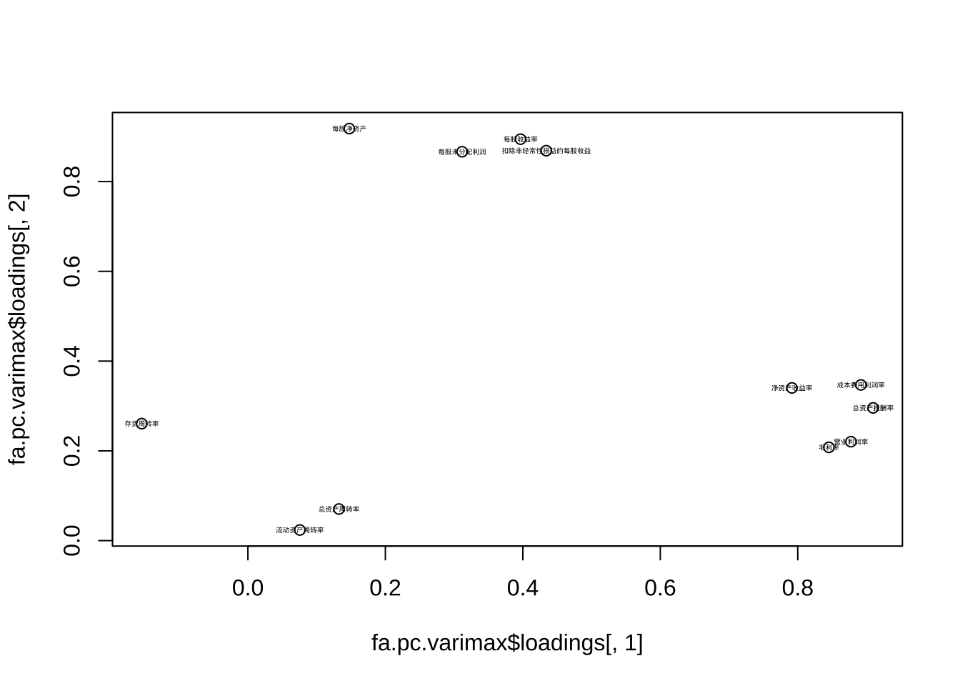

biplot(fa.pc.varimax$scores[,1:2],
       fa.pc.varimax$loadings[,1:2])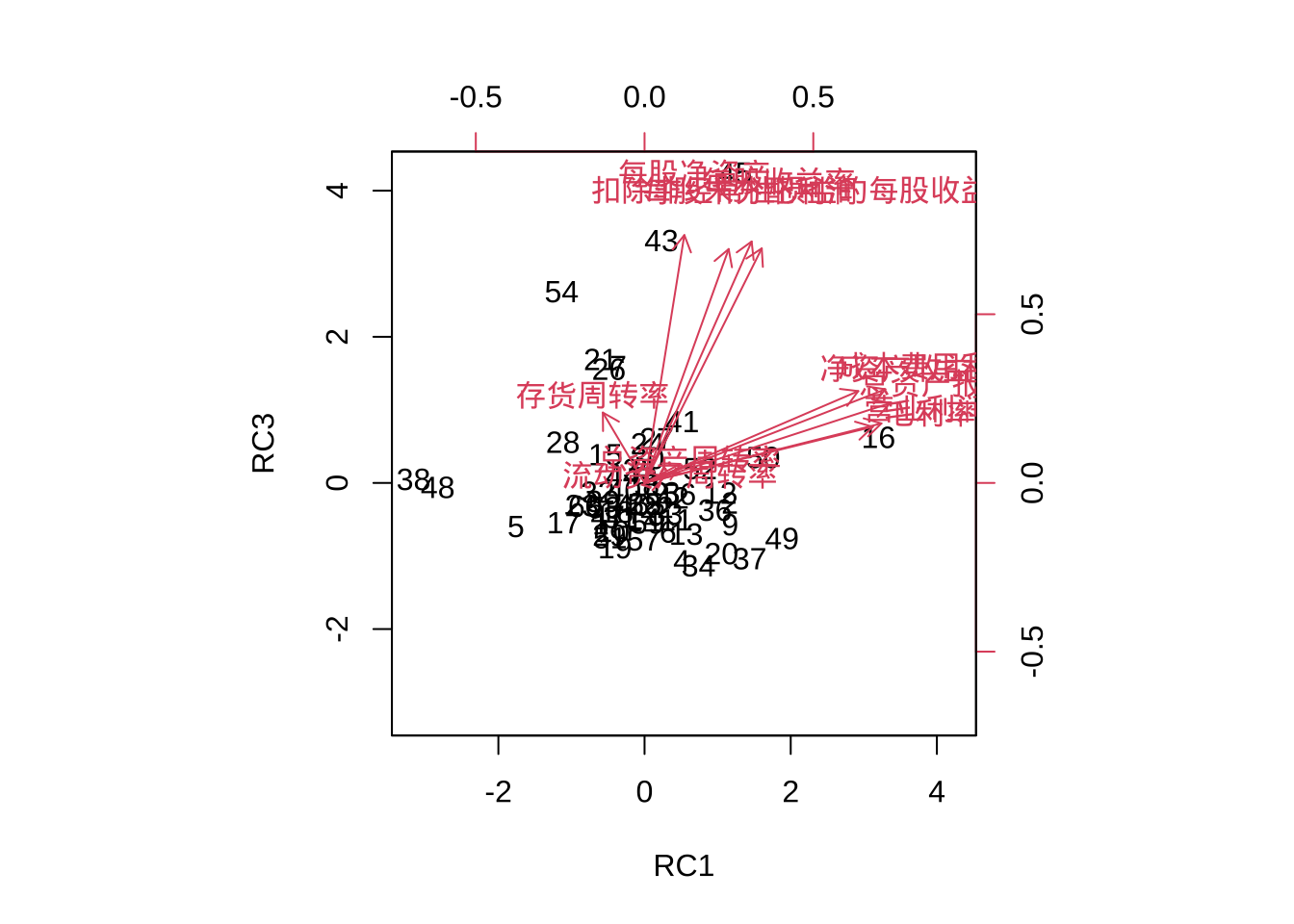

library(scatterplot3d)
scatterplot3d(fa.pc.varimax$loadings, 
              main="3D factor loadings", 
              color=c(rep(1,3), rep(2,5), rep(3,4)),
              pch=20)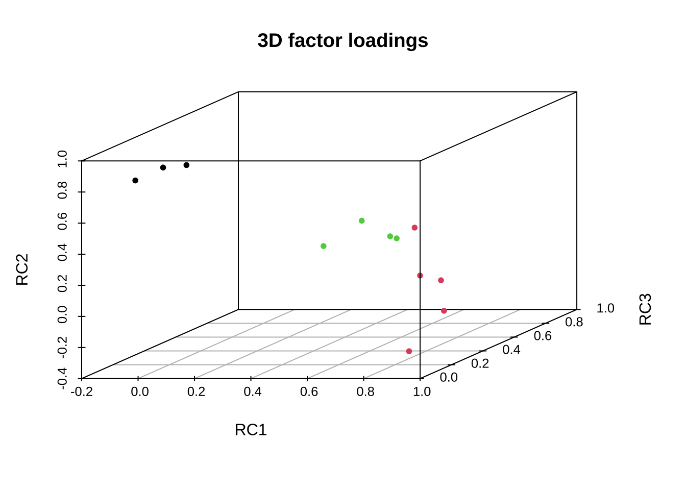

scatterplot3d(fa.pc.varimax$scores, 
              main="3D factor scores",
              pch=20)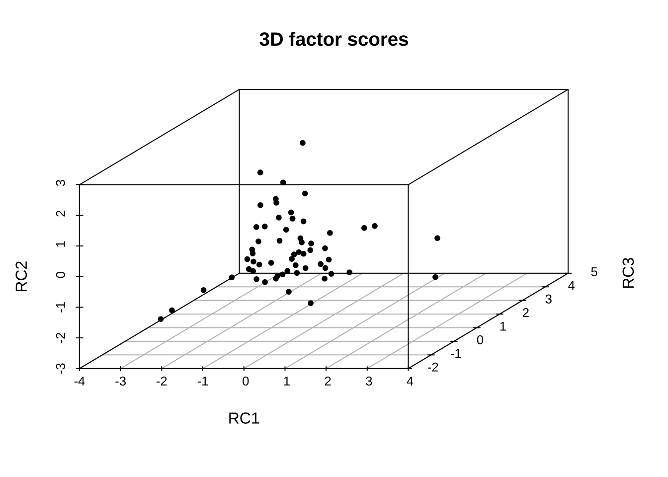

fa.pc.varimax$Call

principal(r = case7_1[-1], nfactors = 3, rotate = "varimax")

fa.pc.varimax <- principal(case7_1[-1], nfactors = 3,
                           rotate = "varimax",
                           method = "wls")



fa.pc.varimax$scores %>% 
  data.frame() %>% 
  cbind(case7_1$证券名称,.) %>% 
  select(1:2) %>% 
  arrange(desc(RC1))%>% 
  head()

  case7_1$证券名称      RC1
1           新坐标 3.200275
2         浙江仙通 1.880036
3         岱美股份 1.622674
4         继峰股份 1.438485
5         兆丰股份 1.240185
6         中原内配 1.169983

fa.pc.varimax$scores %>% 
  data.frame() %>% 
  cbind(case7_1$证券名称,.) %>% 
  select(1,3) %>% 
  arrange(desc(RC3))%>% 
  head()

  case7_1$证券名称      RC3
1         兆丰股份 4.239737
2         苏威孚Ｂ 3.316791
3         华域汽车 2.615909
4         德尔股份 1.690839
5         越博动力 1.594501
6         宁波华翔 1.556167

fa.pc.varimax$scores %>% 
  data.frame() %>% 
  cbind(case7_1$证券名称,.) %>%
  select(1,4) %>%  
  arrange(desc(RC2)) %>% 
  head()

  case7_1$证券名称      RC2
1         东风科技 2.567504
2         华域汽车 2.314485
3         亚普股份 2.308875
4         众泰汽车 1.693966
5         交运股份 1.556585
6         凌云股份 1.353060

教材P160 习题7.7

library(readxl)
library(tidyverse)
ex7_7 <- read_excel("ex6.6.xls") %>% 
  rename(工业废水排放量 = x1, 
         工业化学需氧量 = x2,
         工业氨氮排放量 = x3, 
         城镇生活污水排放量 = x4, 
         生活化学需氧量排放量 = x5, 
         生活氨氮排放量 = x6
         )

rownames(ex7_7) <- ex7_7$城市

fa.pc.varimax <- principal(ex7_7[-1], nfactors = 2,
                          rotate = "varimax")
fa.pc.varimax

Principal Components Analysis
Call: principal(r = ex7_7[-1], nfactors = 2, rotate = "varimax")
Standardized loadings (pattern matrix) based upon correlation matrix
                      RC1  RC2   h2    u2 com
工业废水排放量       0.77 0.38 0.74 0.257 1.5
工业化学需氧量       0.53 0.81 0.93 0.068 1.7
工业氨氮排放量       0.10 0.96 0.93 0.069 1.0
城镇生活污水排放量   0.94 0.01 0.89 0.114 1.0
生活化学需氧量排放量 0.85 0.30 0.81 0.185 1.2
生活氨氮排放量       0.88 0.35 0.91 0.092 1.3

                       RC1  RC2
SS loadings           3.28 1.93
Proportion Var        0.55 0.32
Cumulative Var        0.55 0.87
Proportion Explained  0.63 0.37
Cumulative Proportion 0.63 1.00

Mean item complexity =  1.3
Test of the hypothesis that 2 components are sufficient.

The root mean square of the residuals (RMSR) is  0.06 
 with the empirical chi square  1.82  with prob <  0.77 

Fit based upon off diagonal values = 0.99

print(fa.pc.varimax$loadings, digits = 3, cutoff = 0.5,sort = T)


Loadings:
                     RC1   RC2  
工业废水排放量       0.774      
城镇生活污水排放量   0.941      
生活化学需氧量排放量 0.851      
生活氨氮排放量       0.884      
工业化学需氧量       0.531 0.806
工业氨氮排放量             0.960

                 RC1   RC2
SS loadings    3.283 1.931
Proportion Var 0.547 0.322
Cumulative Var 0.547 0.869

fa.pc.promax <- principal(ex7_7[-1], nfactors = 2,
                           rotate = "promax")
fa.pc.promax

Principal Components Analysis
Call: principal(r = ex7_7[-1], nfactors = 2, rotate = "promax")
Standardized loadings (pattern matrix) based upon correlation matrix
                       RC1   RC2   h2    u2 com
工业废水排放量        0.75  0.18 0.74 0.257 1.1
工业化学需氧量        0.33  0.75 0.93 0.068 1.4
工业氨氮排放量       -0.22  1.06 0.93 0.069 1.1
城镇生活污水排放量    1.07 -0.29 0.89 0.114 1.2
生活化学需氧量排放量  0.87  0.06 0.81 0.185 1.0
生活氨氮排放量        0.89  0.11 0.91 0.092 1.0

                       RC1  RC2
SS loadings           3.40 1.82
Proportion Var        0.57 0.30
Cumulative Var        0.57 0.87
Proportion Explained  0.65 0.35
Cumulative Proportion 0.65 1.00

 With component correlations of 
     RC1  RC2
RC1 1.00 0.54
RC2 0.54 1.00

Mean item complexity =  1.1
Test of the hypothesis that 2 components are sufficient.

The root mean square of the residuals (RMSR) is  0.06 
 with the empirical chi square  1.82  with prob <  0.77 

Fit based upon off diagonal values = 0.99

print(fa.pc.promax$loadings, digits = 3, cutoff = 0.5,sort = T)


Loadings:
                     RC1    RC2   
工业废水排放量        0.753       
城镇生活污水排放量    1.068       
生活化学需氧量排放量  0.867       
生活氨氮排放量        0.887       
工业化学需氧量               0.745
工业氨氮排放量               1.064

                 RC1   RC2
SS loadings    3.401 1.823
Proportion Var 0.567 0.304
Cumulative Var 0.567 0.871

biplot(fa.pc.promax)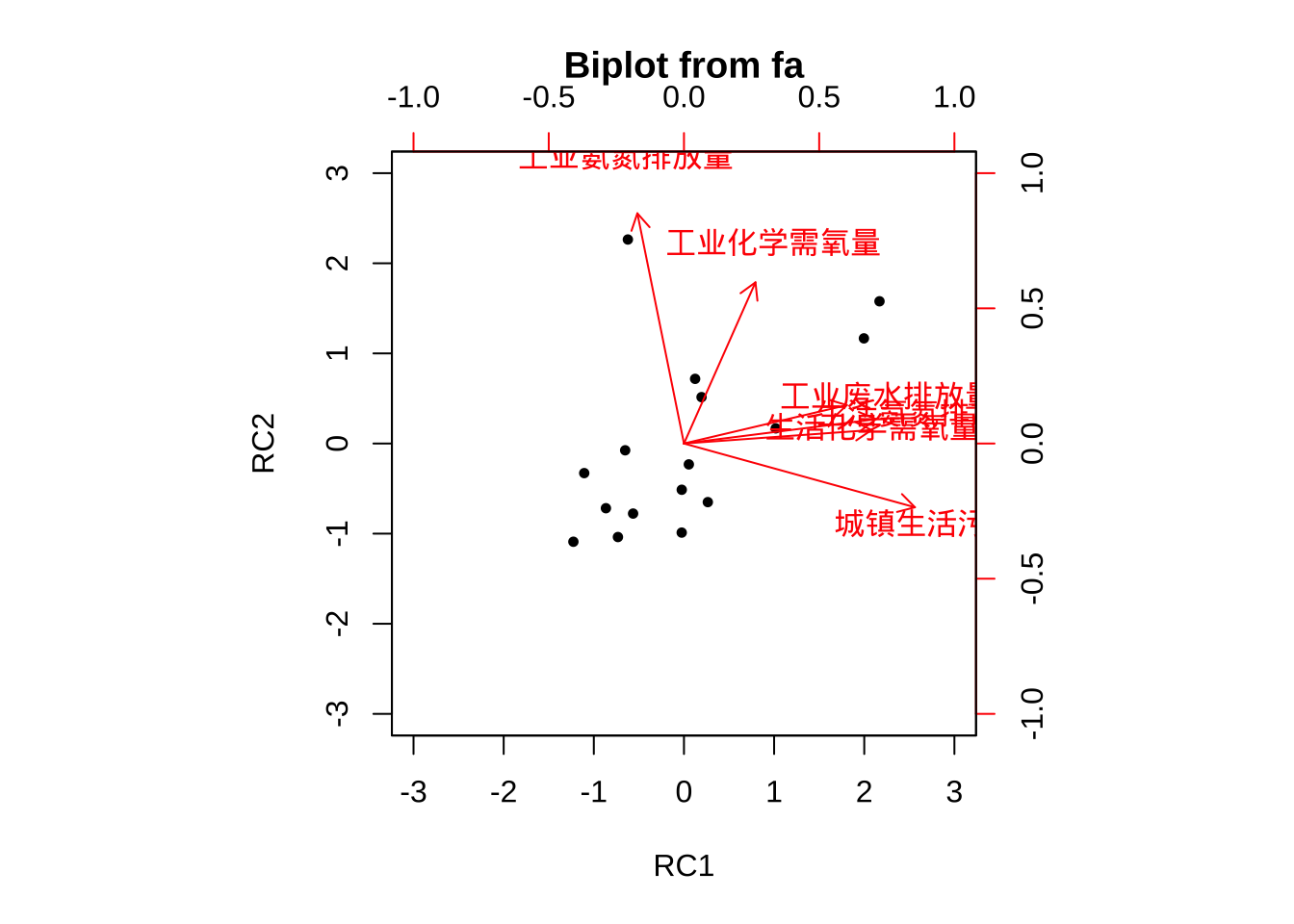

biplot(fa.pc.promax$scores[,1:2],
       fa.pc.promax$loadings[,1:2],
       xlim = c(-3,3),
       ylim = c(-3,3),
       xlabs = ex7_7$城市)
       
abline(v = 0, h = 0, lty = 2, col = "grey25")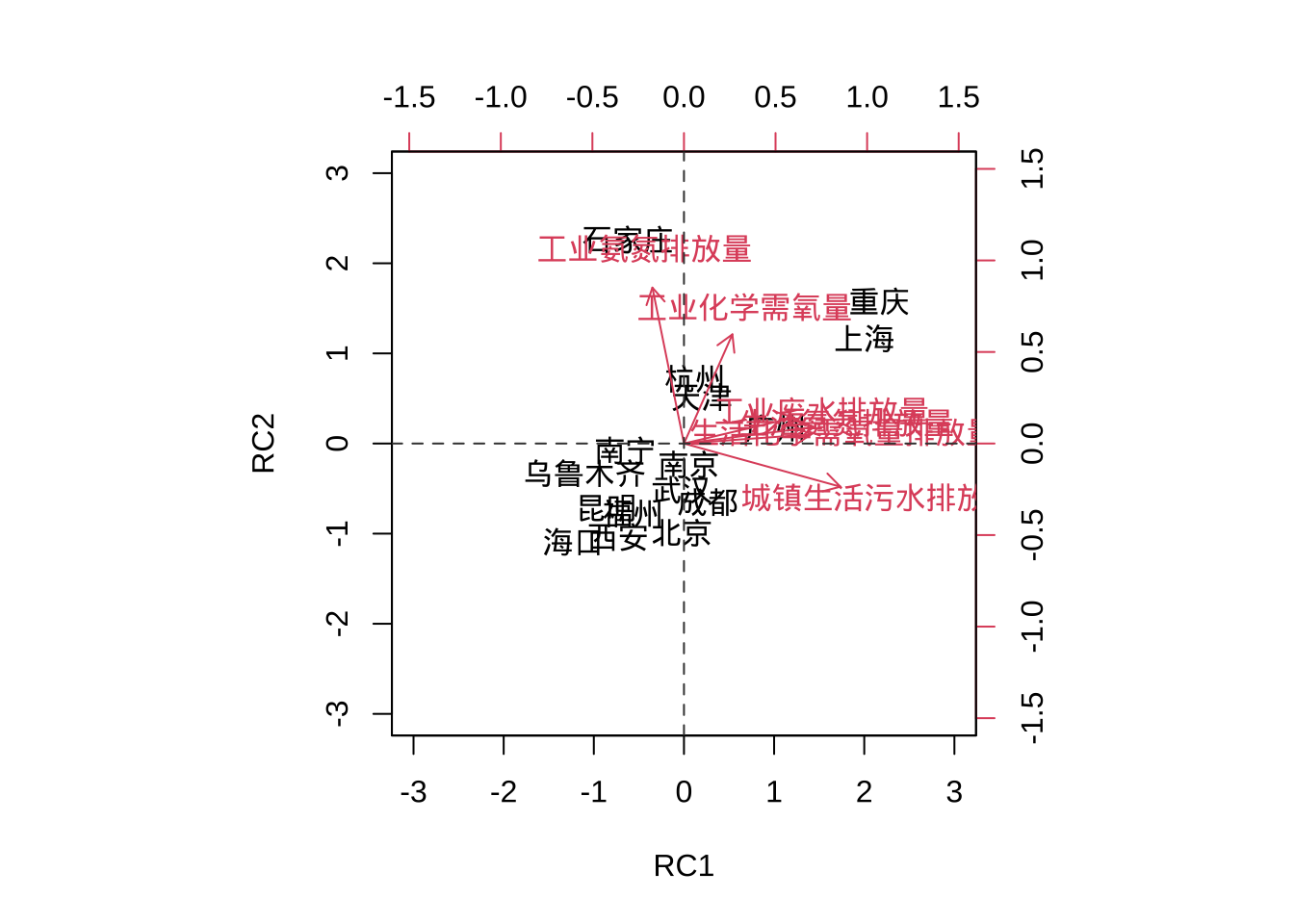

fa.pc.promax$scores %>% 
  round(3) %>% 
  cbind(ex7_7$城市,.) %>% 
  data.frame() %>% 
  arrange(desc(RC1)) %>% 
  head()

    V1   RC1   RC2
1 重庆 2.169 1.578
2 上海 1.996 1.167
3 广州 1.018 0.168
4 成都 0.265 -0.65
5 天津 0.195 0.515
6 杭州 0.124 0.718

fa.pc.promax$scores %>% 
  round(3) %>% 
  cbind(ex7_7$城市,.) %>% 
  data.frame() %>% 
  arrange(desc(RC2)) %>% 
  head()

      V1    RC1   RC2
1 石家庄 -0.622 2.264
2   重庆  2.169 1.578
3   上海  1.996 1.167
4   杭州  0.124 0.718
5   天津  0.195 0.515
6   广州  1.018 0.168