library(tidyverse)
library(psych)

fa.pc.varimax <- car_sales %>% select(engine_s:mpg) %>%
  principal(nfactors = 2,
            rotate = "varimax")

fa.pc.varimax
Principal Components Analysis
Call: principal(r = ., nfactors = 2, rotate = "varimax")
Standardized loadings (pattern matrix) based upon correlation matrix
           RC1   RC2   h2   u2 com
engine_s  0.88  0.32 0.87 0.13 1.3
horsepow  0.89  0.09 0.80 0.20 1.0
wheelbas  0.19  0.94 0.91 0.09 1.1
width     0.52  0.69 0.75 0.25 1.9
length    0.23  0.89 0.84 0.16 1.1
curb_wgt  0.72  0.58 0.85 0.15 1.9
fuel_cap  0.64  0.59 0.76 0.24 2.0
mpg      -0.80 -0.37 0.78 0.22 1.4

                       RC1  RC2
SS loadings           3.49 3.06
Proportion Var        0.44 0.38
Cumulative Var        0.44 0.82
Proportion Explained  0.53 0.47
Cumulative Proportion 0.53 1.00

Mean item complexity =  1.5
Test of the hypothesis that 2 components are sufficient.

The root mean square of the residuals (RMSR) is  0.07
 with the empirical chi square  38.95  with prob <  2e-04

Fit based upon off diagonal values = 0.99
print(fa.pc.varimax$loadings, digits = 3, cutoff = 0.5,sort = T)
Loadings:
         RC1    RC2
engine_s  0.876
horsepow  0.888
curb_wgt  0.722  0.577
fuel_cap  0.644  0.586
mpg      -0.803
wheelbas         0.935
width     0.517  0.693
length           0.888

                 RC1   RC2
SS loadings    3.493 3.063
Proportion Var 0.437 0.383
Cumulative Var 0.437 0.819
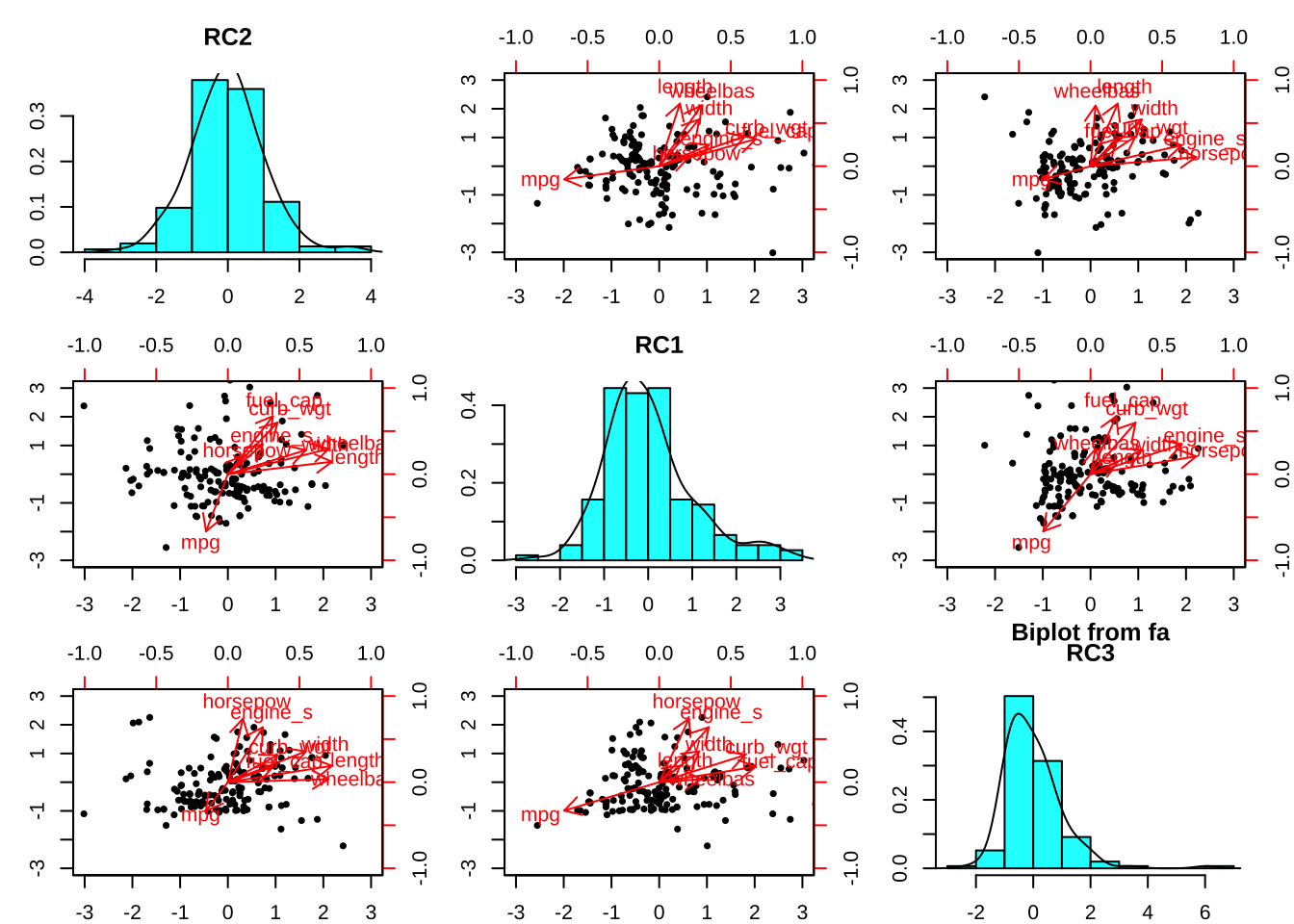
fa.pc.varimax <- car_sales %>% select(engine_s:mpg) %>%
  principal(nfactors = 3,
            rotate = "varimax")

fa.pc.varimax
Principal Components Analysis
Call: principal(r = ., nfactors = 3, rotate = "varimax")
Standardized loadings (pattern matrix) based upon correlation matrix
           RC2   RC1   RC3   h2    u2 com
engine_s  0.31  0.43  0.80 0.92 0.084 1.9
horsepow  0.13  0.26  0.92 0.93 0.066 1.2
wheelbas  0.88  0.37  0.04 0.91 0.090 1.3
width     0.68  0.35  0.45 0.78 0.216 2.3
length    0.91  0.18  0.24 0.91 0.085 1.2
curb_wgt  0.43  0.75  0.39 0.90 0.099 2.2
fuel_cap  0.39  0.84  0.22 0.91 0.085 1.6
mpg      -0.19 -0.83 -0.41 0.89 0.107 1.6

                       RC2  RC1  RC3
SS loadings           2.55 2.50 2.12
Proportion Var        0.32 0.31 0.26
Cumulative Var        0.32 0.63 0.90
Proportion Explained  0.36 0.35 0.30
Cumulative Proportion 0.36 0.70 1.00

Mean item complexity =  1.7
Test of the hypothesis that 3 components are sufficient.

The root mean square of the residuals (RMSR) is  0.03
 with the empirical chi square  8.66  with prob <  0.28

Fit based upon off diagonal values = 1
print(fa.pc.varimax$loadings, digits = 3, cutoff = 0.5,sort = T)
Loadings:
         RC2    RC1    RC3
wheelbas  0.879
width     0.680
length    0.908
curb_wgt         0.748
fuel_cap         0.842
mpg             -0.829
engine_s                0.797
horsepow                0.922

                 RC2   RC1   RC3
SS loadings    2.550 2.500 2.119
Proportion Var 0.319 0.312 0.265
Cumulative Var 0.319 0.631 0.896
library(tidyverse)
data <- cbind(car_sales, fa.pc.varimax$scores)
data <- data %>% mutate(suv = if_else(type == 1, 1,0))
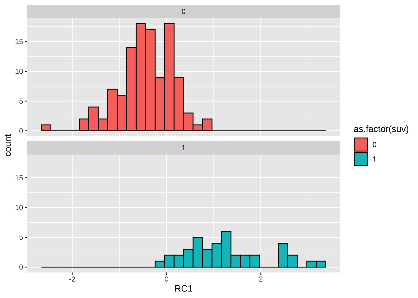
# RC1,其值越大,代表车重大、油箱容积大、耗油越高(SUV)
data %>% ggplot(aes(RC1, fill = as.factor(suv)))+
geom_histogram(col = 1)+
facet_wrap(~ suv,ncol = 1)
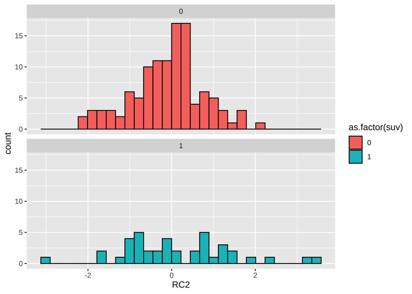
# RC2,其值越大,代表车子轮距、车宽、车长大

data %>% ggplot(aes(RC2, fill = as.factor(suv)))+
  geom_histogram(col = 1)+
  facet_wrap(~ suv,ncol = 1)
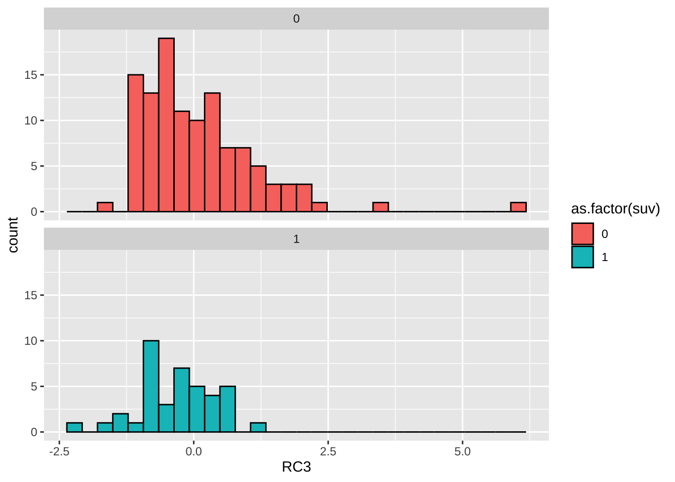
# RC3,动力性能

data %>% ggplot(aes(RC3, fill = as.factor(suv)))+
  geom_histogram(col = 1)+
  facet_wrap(~ suv,ncol = 1)
eq1 <- lm(price ~ RC1 +RC2 +RC3, data)
summary(eq1)
Call:
lm(formula = price ~ RC1 + RC2 + RC3, data = data)

Residuals:
    Min      1Q  Median      3Q     Max
-21.468  -5.049  -0.936   2.972  36.978

Coefficients:
            Estimate Std. Error t value Pr(>|t|)
(Intercept)  27.4646     0.7014  39.156  < 2e-16 ***
RC1           4.3130     0.6999   6.162 6.47e-09 ***
RC2          -1.0709     0.7001  -1.530    0.128
RC3          10.6574     0.7036  15.148  < 2e-16 ***
---
Signif. codes:  0 '***' 0.001 '**' 0.01 '*' 0.05 '.' 0.1 ' ' 1

Residual standard error: 8.643 on 148 degrees of freedom
  (5 observations deleted due to missingness)
Multiple R-squared:  0.6479,    Adjusted R-squared:  0.6407
F-statistic: 90.76 on 3 and 148 DF,  p-value: < 2.2e-16
eq2 <- lm(resale ~ RC1 +RC2 +RC3, data)
summary(eq2)
Call:
lm(formula = resale ~ RC1 + RC2 + RC3, data = data)

Residuals:
    Min      1Q  Median      3Q     Max
-14.680  -4.848  -1.442   2.978  30.519

Coefficients:
            Estimate Std. Error t value Pr(>|t|)
(Intercept)  18.5900     0.7066  26.310  < 2e-16 ***
RC1           3.0571     0.7242   4.222  4.9e-05 ***
RC2          -2.1020     0.6729  -3.124  0.00227 **
RC3           7.5295     0.6661  11.303  < 2e-16 ***
---
Signif. codes:  0 '***' 0.001 '**' 0.01 '*' 0.05 '.' 0.1 ' ' 1

Residual standard error: 7.639 on 114 degrees of freedom
  (39 observations deleted due to missingness)
Multiple R-squared:  0.5742,    Adjusted R-squared:  0.563
F-statistic: 51.25 on 3 and 114 DF,  p-value: < 2.2e-16
eq3 <- lm(sales ~ RC1 +RC2 +RC3, data)
summary(eq3)
Call:
lm(formula = sales ~ RC1 + RC2 + RC3, data = data)

Residuals:
   Min     1Q Median     3Q    Max
-88.46 -35.92 -18.67  20.10 397.87

Coefficients:
             Estimate Std. Error t value Pr(>|t|)
(Intercept)  53.30585    5.08555  10.482  < 2e-16 ***
RC1           0.05693    5.08494   0.011  0.99108
RC2          25.16954    5.09264   4.942 2.05e-06 ***
RC3         -14.56111    5.11090  -2.849  0.00501 **
---
Signif. codes:  0 '***' 0.001 '**' 0.01 '*' 0.05 '.' 0.1 ' ' 1

Residual standard error: 62.88 on 149 degrees of freedom
  (4 observations deleted due to missingness)
Multiple R-squared:  0.1808,    Adjusted R-squared:  0.1643
F-statistic: 10.96 on 3 and 149 DF,  p-value: 1.508e-06
 点击下载数据文件: car_sales.xlsx