8 对应分析习题答案

Author

Li Zongzhang

Published

October 30, 2025

习题2: 收入&满意度

Image Description

提示：数据请自行录入，可在EXCEL录入好后，再导入R。

要求： 2.1 对行变量和列变量进行独立性检验，独立性检验的卡方检验统计量是多少？P值是什么，你的检验结论是什么？

2.2 绘制碎石图。你提取几个维度？每个维度的贡献分别是多少？

2.3 绘制对应分析图。

2.4 绘制行变量的contribution、cos2的图像。

2.5 绘制列变量的contribution、cos2的图像。

2.6 从图中可以发现哪些组别关系紧密？

创建列联表的数据框

#创建列联表的数据框
ex2 <- data.frame(
  very_dissatisfied = c(42,35,13,7,3),
  somewhat_dissatified = c(82,62,28,18,7),
  somewhat_satisfied = c(67,165,92,54,32),
  very_satisfied = c(55, 118,81,75,54)
)

#给ex2添加行名，以便在图中能添加标签
rownames(ex2) <- c("less than 10k", "10k-30k",
                   "30k-50k", "50k-100k", "more than 100k")
ex2

               very_dissatisfied somewhat_dissatified somewhat_satisfied
less than 10k                 42                   82                 67
10k-30k                       35                   62                165
30k-50k                       13                   28                 92
50k-100k                       7                   18                 54
more than 100k                 3                    7                 32
               very_satisfied
less than 10k              55
10k-30k                   118
30k-50k                    81
50k-100k                   75
more than 100k             54

2.1 独立性检验

#2.1 对行变量和列变量进行独立性检验，独立性检验的卡方检验统计量是多少？P值是什么，你的检验结论是什么？

chisq.test(ex2)


    Pearson's Chi-squared test

data:  ex2
X-squared = 118.1, df = 12, p-value < 2.2e-16

#卡方检验统计量是118.1, P值接近于0。在0.01的显著性水平下，拒绝“收入等级和满意度等级相互独立”的原假设。

2.2 绘制碎石图

#2.2 绘制碎石图。你提取几个维度？每个维度的贡献分别是多少？

library(FactoMineR)
res.ca <- CA(ex2, graph = FALSE)

#绘制scree plot
library(factoextra)
fviz_screeplot(res.ca, addlabels = TRUE, ylim = c(0, 100))

Warning in geom_bar(stat = "identity", fill = barfill, color = barcolor, :
Ignoring empty aesthetic: `width`.

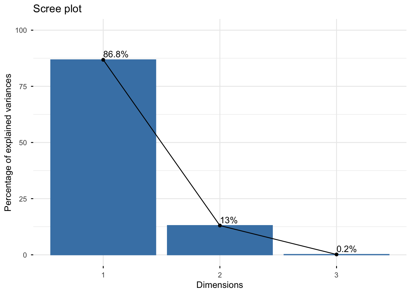
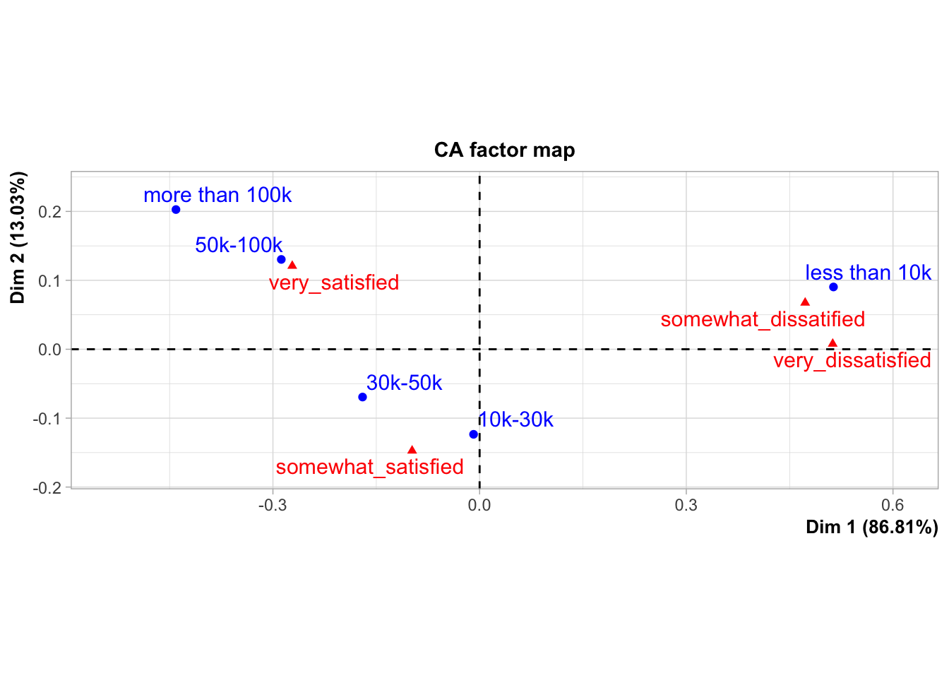
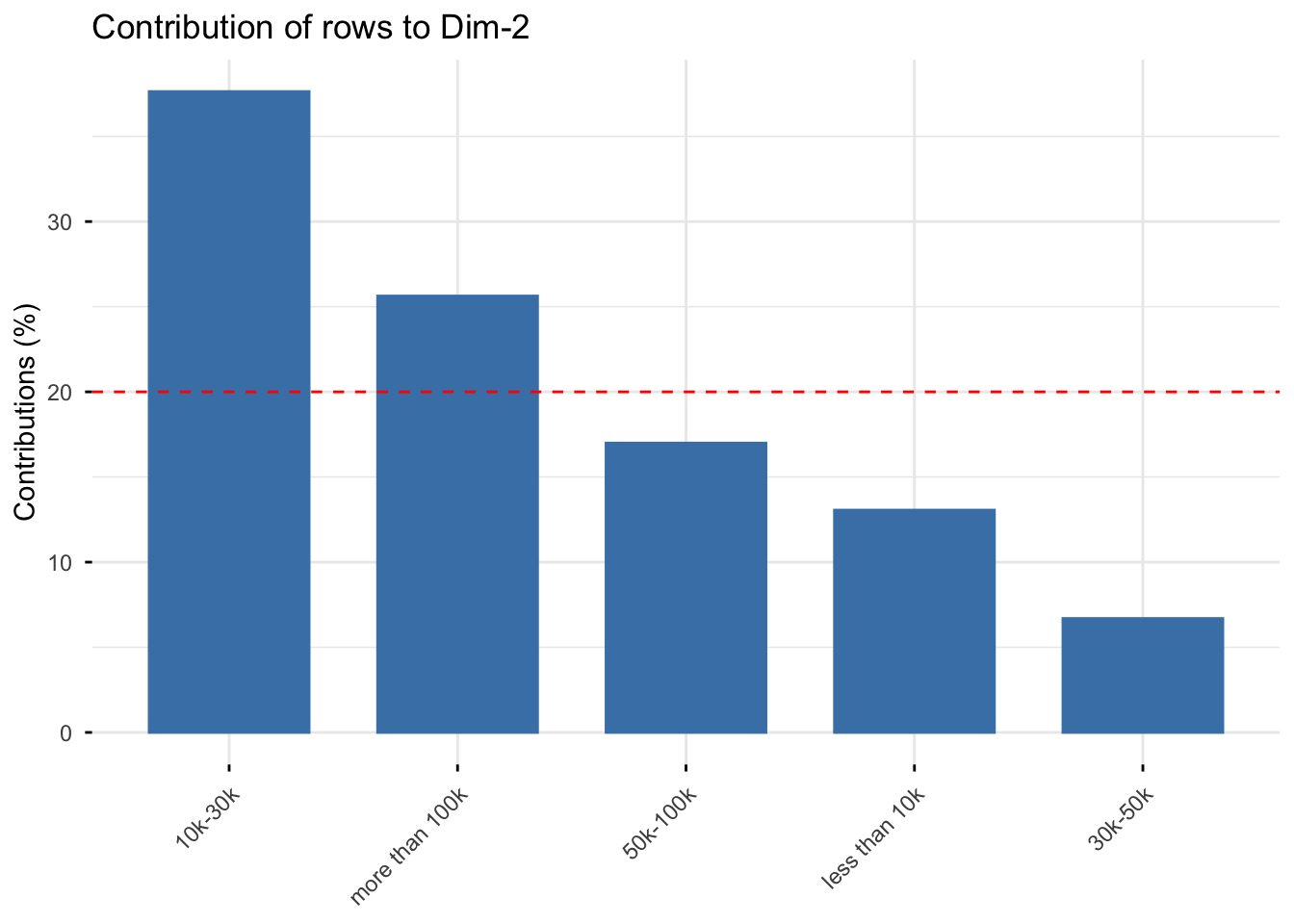
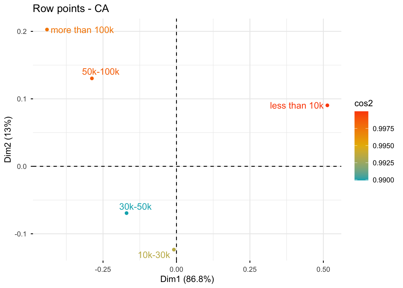
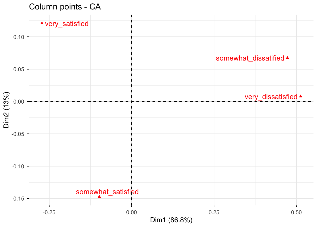
#提取两个维度，维度1的贡献是86.8%， 维度2的贡献是13.0%.

2.3 绘制对应分析图

#2.3 绘制对应分析图
CA(ex2)

**Results of the Correspondence Analysis (CA)**
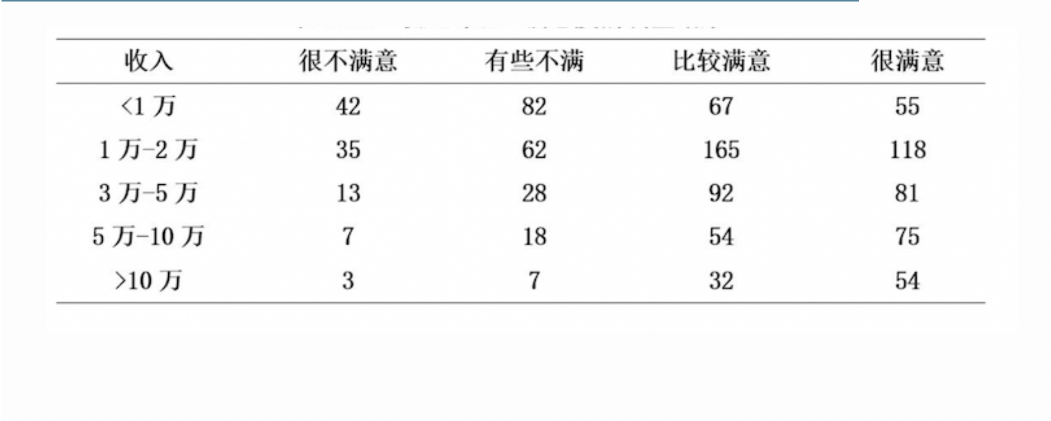
The row variable has  5  categories; the column variable has 4 categories
The chi square of independence between the two variables is equal to 118.0959 (p-value =  1.48029e-19 ).
*The results are available in the following objects:

   name              description                   
1  "$eig"            "eigenvalues"                 
2  "$col"            "results for the columns"     
3  "$col$coord"      "coord. for the columns"      
4  "$col$cos2"       "cos2 for the columns"        
5  "$col$contrib"    "contributions of the columns"
6  "$row"            "results for the rows"        
7  "$row$coord"      "coord. for the rows"         
8  "$row$cos2"       "cos2 for the rows"           
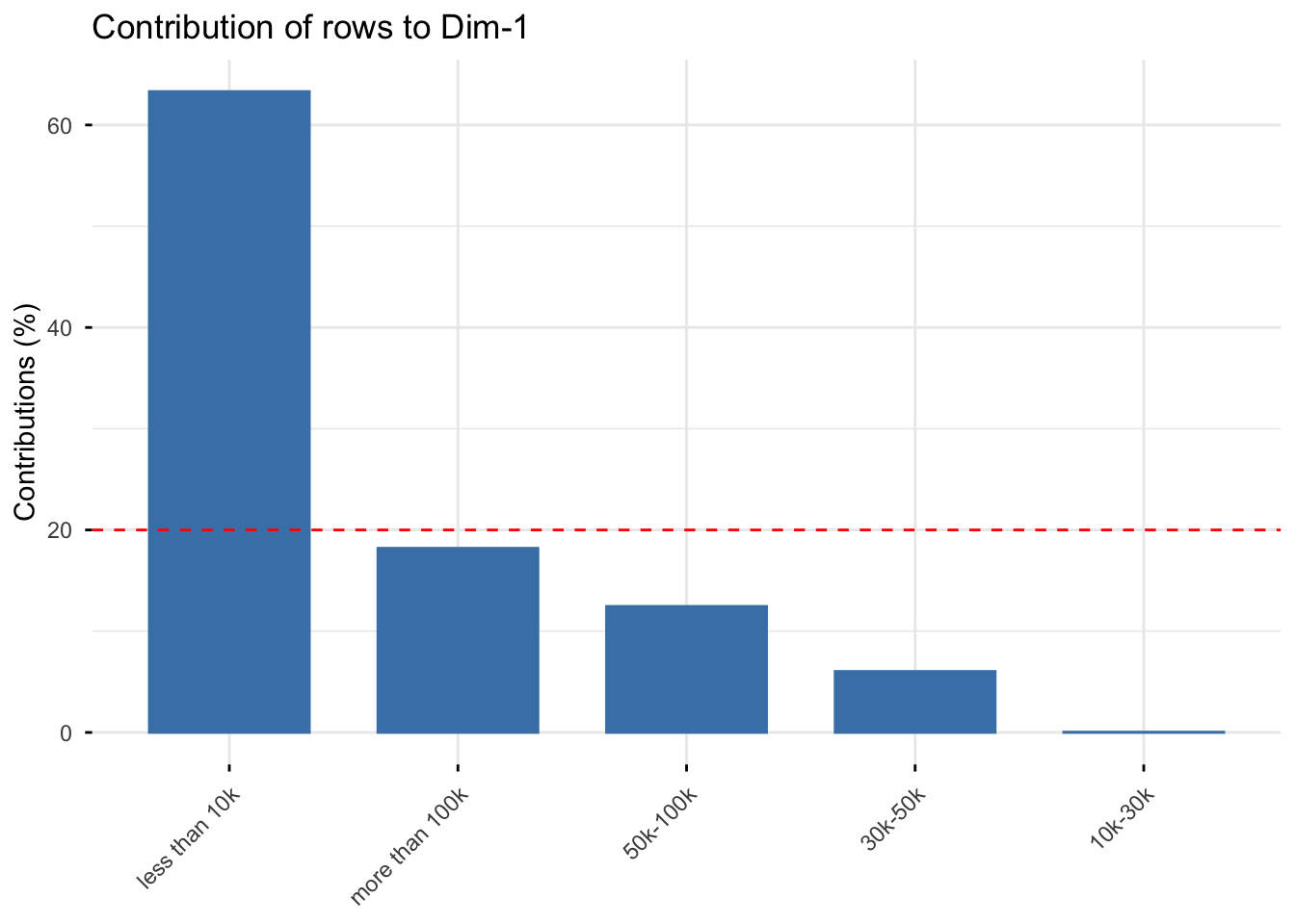
9  "$row$contrib"    "contributions of the rows"   
10 "$call"           "summary called parameters"   
11 "$call$marge.col" "weights of the columns"      
12 "$call$marge.row" "weights of the rows"

2.4 绘制行变量的contribution/cos2图像

#2.4 绘制行变量的contribution的图像。

#行变量对维度1的贡献
fviz_contrib(res.ca, choice = "row", axes = 1)

#行变量对维度2的贡献
fviz_contrib(res.ca, choice = "row", axes = 2)

#2.4 绘制行变量的cos2的图像。
row <- get_ca_row(res.ca)
row$cos2

                     Dim 1      Dim 2        Dim 3
less than 10k  0.969960339 0.03003387 5.791844e-06
10k-30k        0.005022974 0.98842064 6.556387e-03
30k-50k        0.848488225 0.14144329 1.006848e-02
50k-100k       0.828708215 0.16984574 1.446041e-03
more than 100k 0.823408163 0.17415844 2.433397e-03

#维度对行变量的代表性cos2（representation）
fviz_ca_row(res.ca, col.row = "cos2",
             gradient.cols = c("#00AFBB", "#E7B800", "#FC4E07"), 
             repel = TRUE)

2.5 绘制列变量的contribution/cos2图像

#2.5 绘制列变量的contribution的图像。

#列变量对维度1的贡献
fviz_contrib(res.ca, choice = "col", axes = 1)

#列变量对维度2的贡献
fviz_contrib(res.ca, choice = "col", axes = 2)

#2.5 绘制列变量的cos2的图像。
col <- get_ca_col(res.ca)
col$cos2

                         Dim 1        Dim 2        Dim 3
very_dissatisfied    0.9950893 0.0002326784 4.677993e-03
somewhat_dissatified 0.9786700 0.0199298451 1.400105e-03
somewhat_satisfied   0.3068527 0.6930317994 1.155260e-04
very_satisfied       0.8349172 0.1650352038 4.757035e-05

#维度对列变量的代表性cos2（representation）
fviz_ca_col(res.ca, col.row = "cos2",
             gradient.cols = c("#00AFBB", "#E7B800", "#FC4E07"), 
             repel = TRUE)

2.6 结论

从图中可以发现哪些组别关系紧密？

CA(ex2)

**Results of the Correspondence Analysis (CA)**
The row variable has  5  categories; the column variable has 4 categories
The chi square of independence between the two variables is equal to 118.0959 (p-value =  1.48029e-19 ).
*The results are available in the following objects:

   name              description                   
1  "$eig"            "eigenvalues"                 
2  "$col"            "results for the columns"     
3  "$col$coord"      "coord. for the columns"      
4  "$col$cos2"       "cos2 for the columns"        
5  "$col$contrib"    "contributions of the columns"
6  "$row"            "results for the rows"        
7  "$row$coord"      "coord. for the rows"         
8  "$row$cos2"       "cos2 for the rows"           
9  "$row$contrib"    "contributions of the rows"   
10 "$call"           "summary called parameters"   
11 "$call$marge.col" "weights of the columns"      
12 "$call$marge.row" "weights of the rows"

收入介于5万至10万与非常满意关系紧密。

收入小于1万与有些不满意关系紧密。

收入介于1万至3万与有些满意关系紧密。

习题3

Image Description

提示：数据请自行录入，可在EXCEL录入好后，再导入R。

要求： 3.1 对行变量和列变量进行独立性检验，独立性检验的卡方检验统计量是多少？P值是什么，你的检验结论是什么？

3.2 绘制碎石图。你提取几个维度？每个维度的贡献分别是多少？

3.3 绘制对应分析图。

3.4 绘制行变量的contribution、cos2的图像。

3.5 绘制列变量的contribution、cos2的图像。

3.6 从图中可以发现哪些组别关系紧密？

创建列联表的数据框

#创建列联表的数据框
ex3 <- data.frame(
  American = c(37,52,33,6),
  European = c(14,15,15,1),
  Japanese = c(51,44,63,8)
)

#给ex2添加行名，以便在图中能添加标签
rownames(ex3) <- c("Married", "Married with Kids",
                   "Single", "Single with Kids")
ex3

                  American European Japanese
Married                 37       14       51
Married with Kids       52       15       44
Single                  33       15       63
Single with Kids         6        1        8

3.1 独立性检验

#3.1 对行变量和列变量进行独立性检验，独立性检验的卡方检验统计量是多少？P值是什么，你的检验结论是什么？

chisq.test(ex3)


    Pearson's Chi-squared test

data:  ex3
X-squared = 8.3495, df = 6, p-value = 0.2136

chisq.test(ex3)$expected

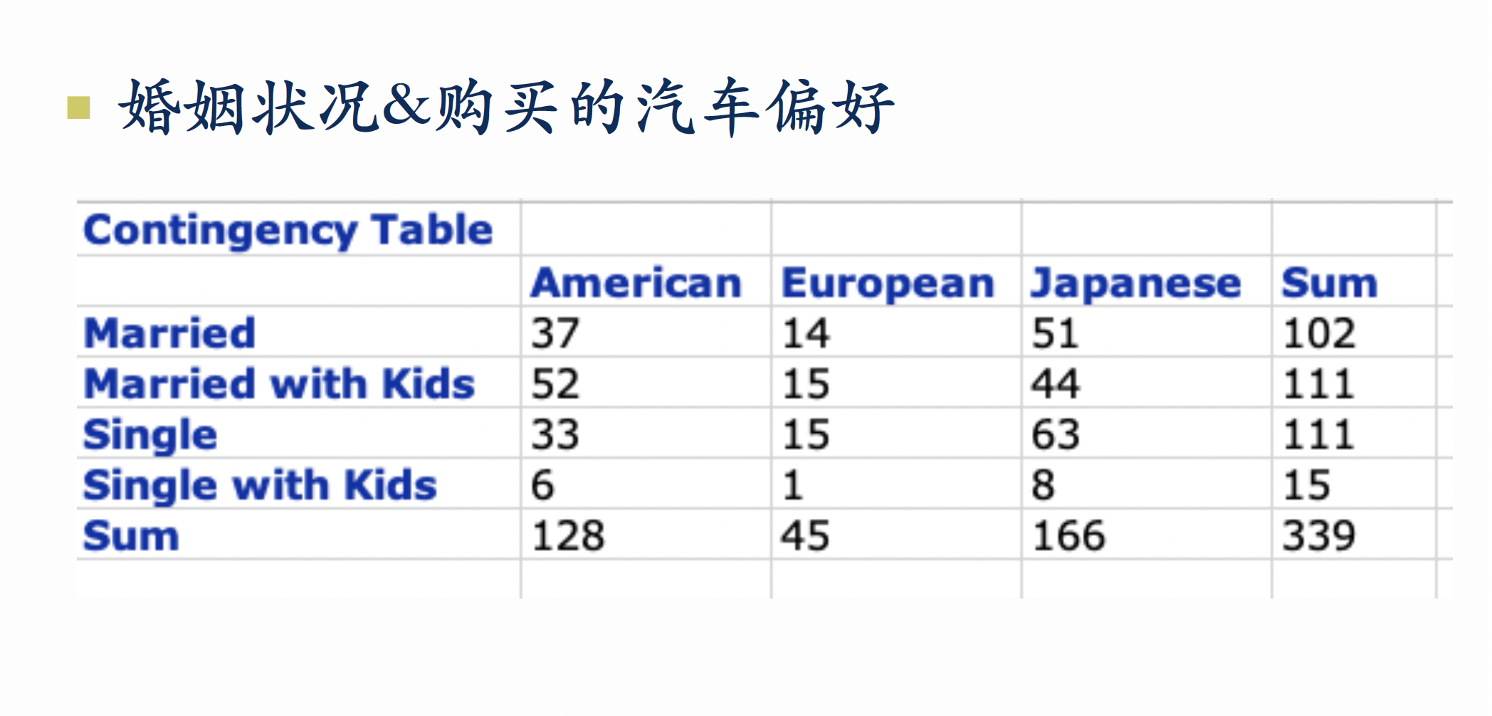
                   American European  Japanese
Married           38.513274 13.53982 49.946903
Married with Kids 41.911504 14.73451 54.353982
Single            41.911504 14.73451 54.353982
Single with Kids   5.663717  1.99115  7.345133

#卡方检验统计量是8.3495, P值等于0.2136。在0.10的显著性水平下，不拒绝“婚姻状况和汽车类型相互独立”的原假设。

#3.1 对行变量和列变量进行独立性检验，独立性检验的卡方检验统计量是多少？P值是什么，你的检验结论是什么？

fisher.test(ex3, workspace = 2e7)


    Fisher's Exact Test for Count Data

data:  ex3
p-value = 0.2145
alternative hypothesis: two.sided

#卡方检验统计量是118.1, P值接近于0。在0.01的显著性水平下，拒绝“收入等级和满意度等级相互独立”的原假设。

3.2 绘制碎石图

#3.2 绘制碎石图。你提取几个维度？每个维度的贡献分别是多少？

library(FactoMineR)
res.ca <- CA(ex3, graph = FALSE)

#绘制scree plot
library(factoextra)
fviz_screeplot(res.ca, addlabels = TRUE, ylim = c(0, 100))

Warning in geom_bar(stat = "identity", fill = barfill, color = barcolor, :
Ignoring empty aesthetic: `width`.

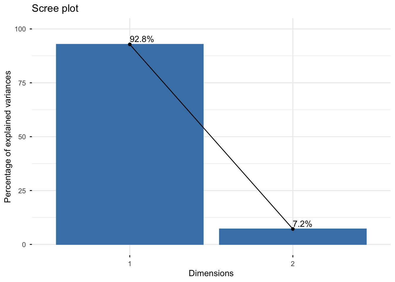
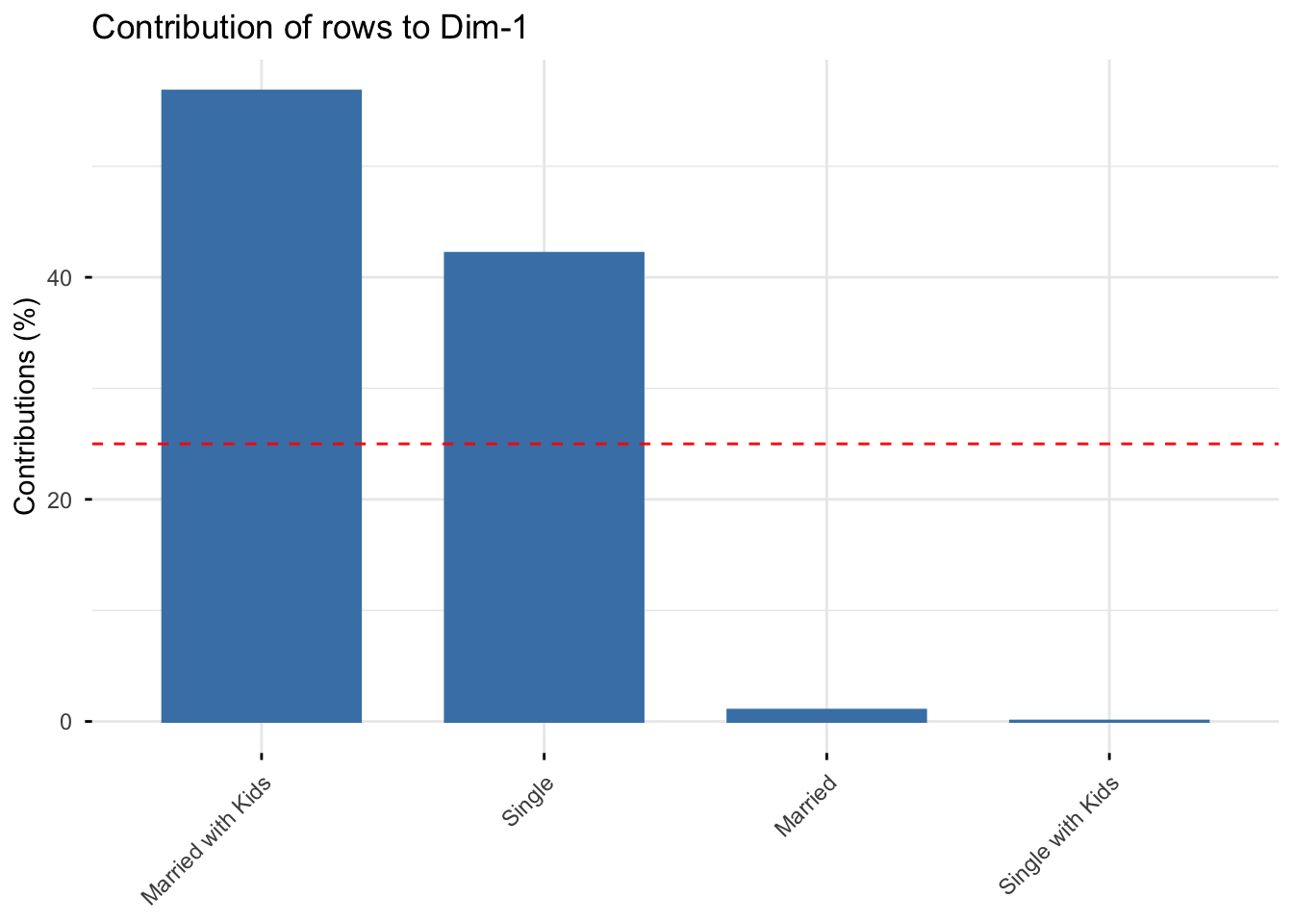
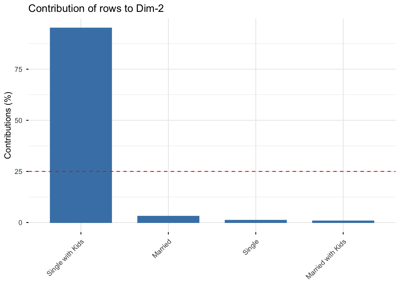
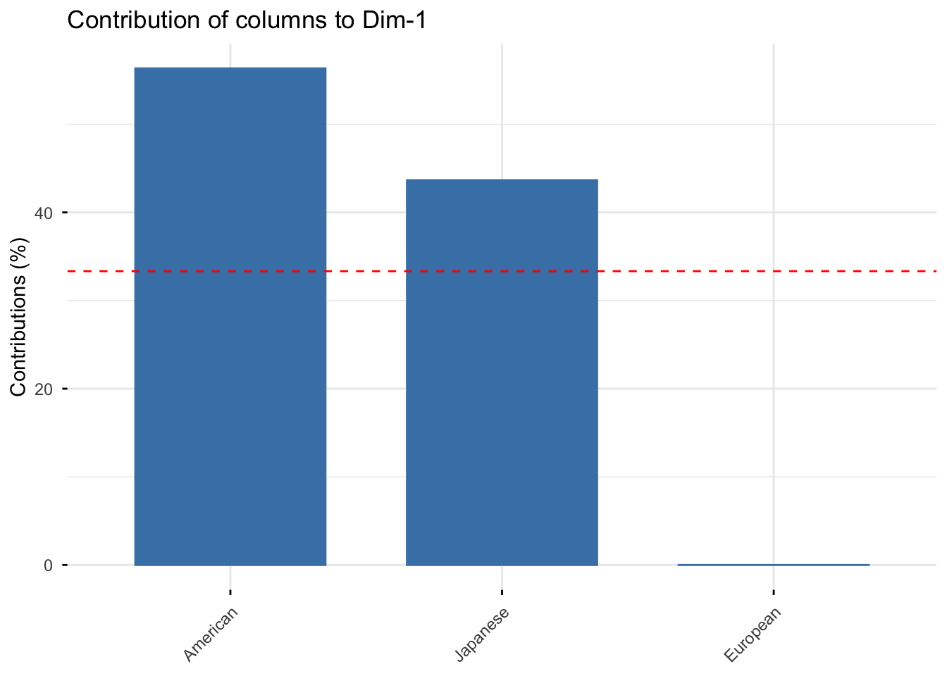
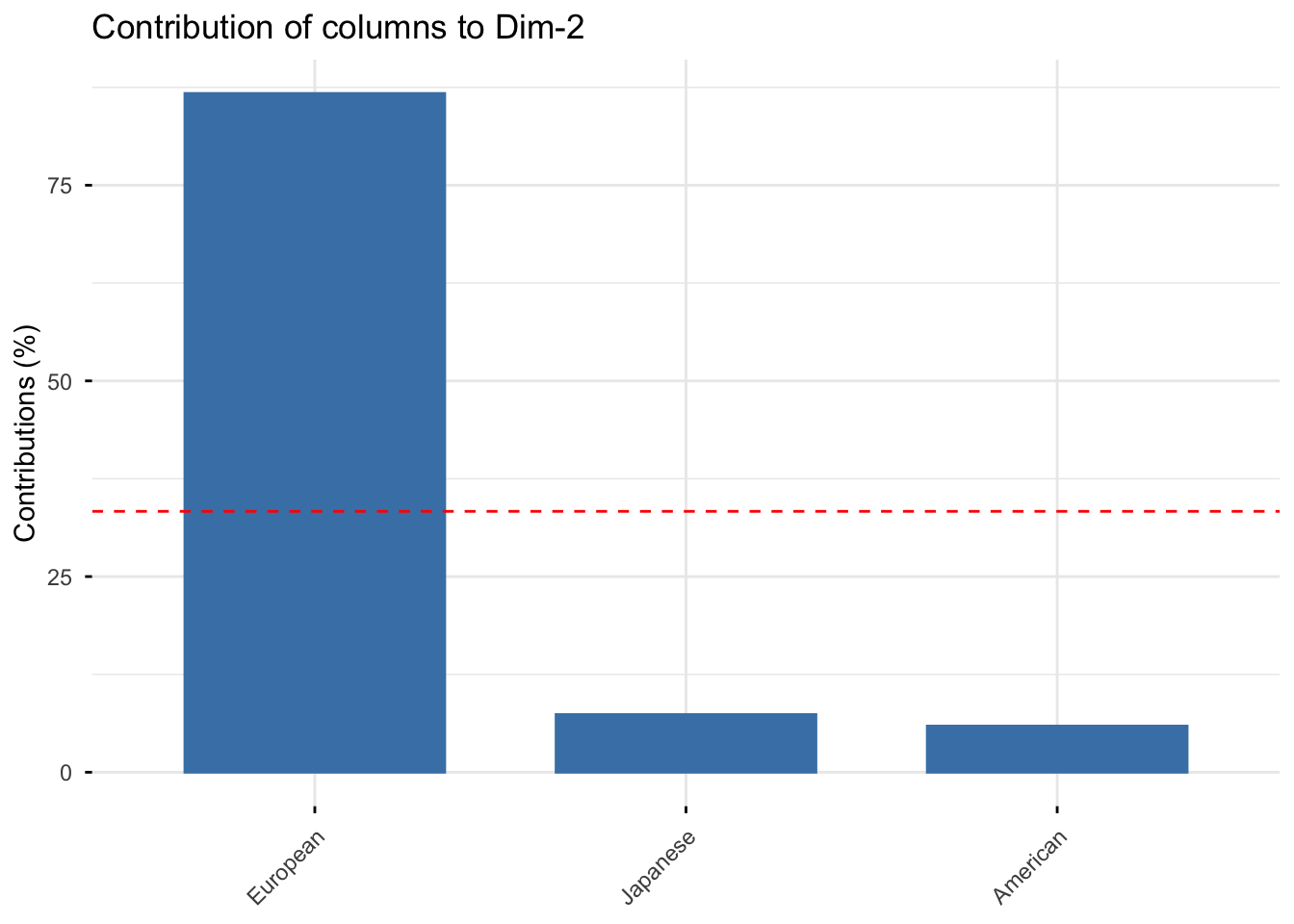
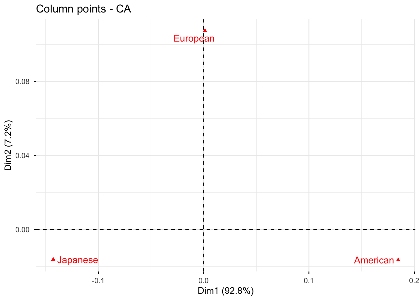
#提取两个维度，维度1的贡献是92.8%， 维度2的贡献是7.2%.

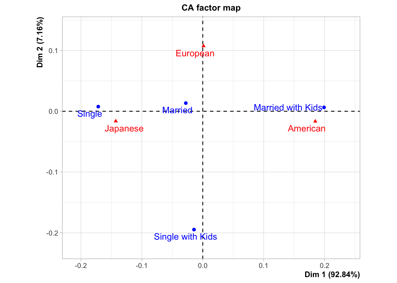
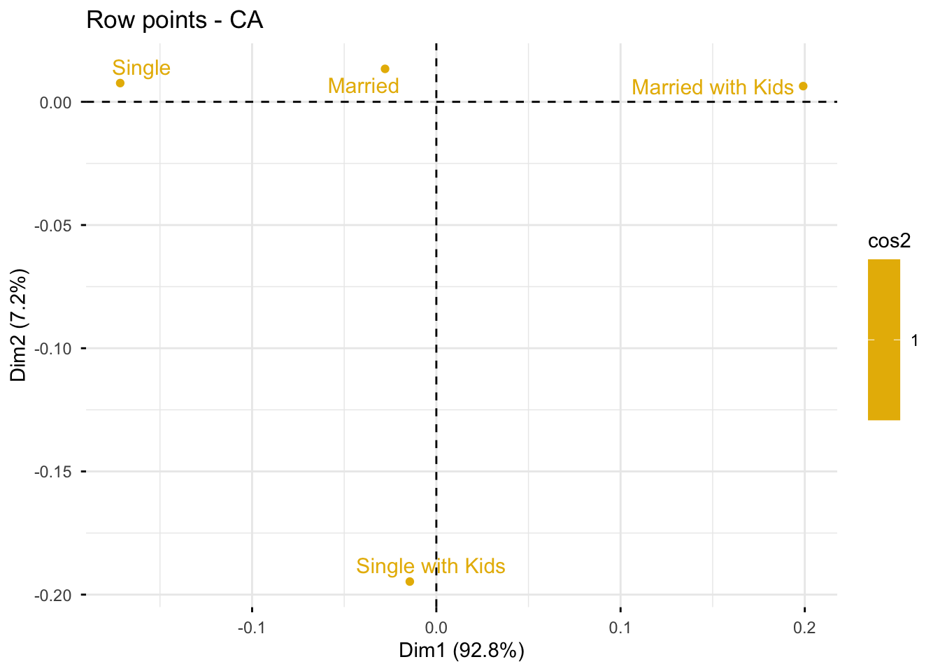
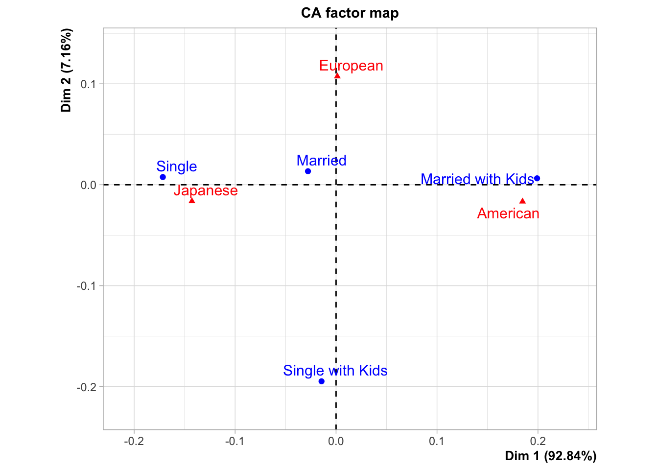
3.3 绘制对应分析图

#2.3 绘制对应分析图
CA(ex3)

**Results of the Correspondence Analysis (CA)**
The row variable has  4  categories; the column variable has 3 categories
The chi square of independence between the two variables is equal to 8.349475 (p-value =  0.2136014 ).
*The results are available in the following objects:

   name              description                   
1  "$eig"            "eigenvalues"                 
2  "$col"            "results for the columns"     
3  "$col$coord"      "coord. for the columns"      
4  "$col$cos2"       "cos2 for the columns"        
5  "$col$contrib"    "contributions of the columns"
6  "$row"            "results for the rows"        
7  "$row$coord"      "coord. for the rows"         
8  "$row$cos2"       "cos2 for the rows"           
9  "$row$contrib"    "contributions of the rows"   
10 "$call"           "summary called parameters"   
11 "$call$marge.col" "weights of the columns"      
12 "$call$marge.row" "weights of the rows"

3.4 绘制行变量的contribution/cos2图像

#3.4 绘制行变量的contribution的图像。

#行变量对维度1的贡献
fviz_contrib(res.ca, choice = "row", axes = 1)

#行变量对维度2的贡献
fviz_contrib(res.ca, choice = "row", axes = 2)

#3.4 绘制行变量的cos2的图像。
row <- get_ca_row(res.ca)
row$cos2

                        Dim 1       Dim 2
Married           0.812065457 0.187934543
Married with Kids 0.998972772 0.001027228
Single            0.998031174 0.001968826
Single with Kids  0.005440686 0.994559314

#维度对行变量的代表性cos2（representation）
fviz_ca_row(res.ca, col.row = "cos2",
             gradient.cols = c("#00AFBB", "#E7B800", "#FC4E07"), 
             repel = TRUE)

3.5 绘制列变量的contribution/cos2图像

#3.5 绘制列变量的contribution的图像。

#列变量对维度1的贡献
fviz_contrib(res.ca, choice = "col", axes = 1)

#列变量对维度2的贡献
fviz_contrib(res.ca, choice = "col", axes = 2)

#3.5 绘制列变量的cos2的图像。
col <- get_ca_col(res.ca)
col$cos2

                Dim 1       Dim 2
American 0.9919873782 0.008012622
European 0.0001441929 0.999855807
Japanese 0.9871383541 0.012861646

#维度对列变量的代表性cos2（representation）
fviz_ca_col(res.ca, col.row = "cos2",
             gradient.cols = c("#00AFBB", "#E7B800", "#FC4E07"), 
             repel = TRUE)

3.6 结论

从图中可以发现哪些组别关系紧密？

**Results of the Correspondence Analysis (CA)**
The row variable has  4  categories; the column variable has 3 categories
The chi square of independence between the two variables is equal to 8.349475 (p-value =  0.2136014 ).
*The results are available in the following objects:

   name              description                   
1  "$eig"            "eigenvalues"                 
2  "$col"            "results for the columns"     
3  "$col$coord"      "coord. for the columns"      
4  "$col$cos2"       "cos2 for the columns"        
5  "$col$contrib"    "contributions of the columns"
6  "$row"            "results for the rows"        
7  "$row$coord"      "coord. for the rows"         
8  "$row$cos2"       "cos2 for the rows"           
9  "$row$contrib"    "contributions of the rows"   
10 "$call"           "summary called parameters"   
11 "$call$marge.col" "weights of the columns"      
12 "$call$marge.row" "weights of the rows"

单身与日系车关系紧密。

已婚有孩子与美系车关系紧密。

已婚、单身有孩子的购车倾向不明显。