广州6大品牌奶茶店消费价格分析

第3-4章

Li Zongzhang

2024-05-16

1 数据和变量

数据来源：大众点评网，广州六大品牌奶茶店

样本容量：336

数据来源：大众点评网，广州6大奶茶品牌

零售价格: retail.price

团购价格：group.price

品牌： brand

区位：area

市区：荔湾，越秀，天河，海珠

近郊：白云，番禺，黄埔

远郊：花都，从化，南沙，增城

2 图形工具

2.1 帕累托图

2.2 分组条形图

2.3 分组直方图

2.4 分组箱线图

2.5 散点图

2.1 帕累托图

library(tidyverse)
library(readxl)
data  <- read_excel("data/top6.xlsx")

library(forcats)
data %>% ggplot(aes(fct_infreq(brand), fill = brand)) + 
  geom_bar() +
  geom_text(stat = "count", aes(label = after_stat(count)), vjust = -0.5)+ 
  scale_y_continuous(limits = c(0,100))+
  guides(x = guide_axis(angle = 45)) +
  labs(x = "品牌", fill = "品牌") +
  theme_bw() +
  theme(text = element_text(size = 15),
        legend.position = "bottom",
        legend.text = element_text(size = 10))

2.2 分组条形图

data %>%
  group_by(area, brand) %>%
  summarise(count = n(), .groups = "drop") %>% 
  mutate(brand_order = paste(brand, area, rank(-count), sep = "_"))  %>% 
  ggplot(aes(reorder(brand_order, -count),
             count, fill = brand)) +
  geom_col()+
  facet_wrap(~ area, scales = "free_x", ncol = 3) +
  geom_text(aes(label = count), vjust = -0.5) +
  scale_x_discrete(labels = function(x) gsub("_.+$", "", x)) + # 移除排序编号
  scale_y_continuous(limits = c(0, 42)) +
  labs(x = "品牌", y = "数量") +
  theme(axis.text.x = element_text(angle = 42, hjust = 1), 
        legend.position = "none")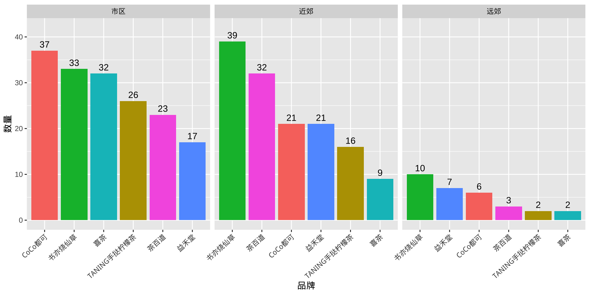

2.3 分组直方图

#按单个定性变量分组
data %>% 
  ggplot(aes(retail.price, fill = brand))+
  geom_histogram(breaks = seq(6, 38, 2))+
  facet_wrap(~brand, ncol = 2) +
  scale_y_continuous(limits = c(0,60))+
  scale_fill_brewer(palette  = "Set1") +
  labs(title = "零售价直方图",
       x = "零售价",
       y = "频数") +
  scale_x_continuous(breaks = seq(6, 36, 4),
                     labels = seq(6, 36, 4)) +
  theme_bw() +
  theme(text = element_text(size = 15),
        legend.position = "bottom",
        legend.text = element_text(size = 10))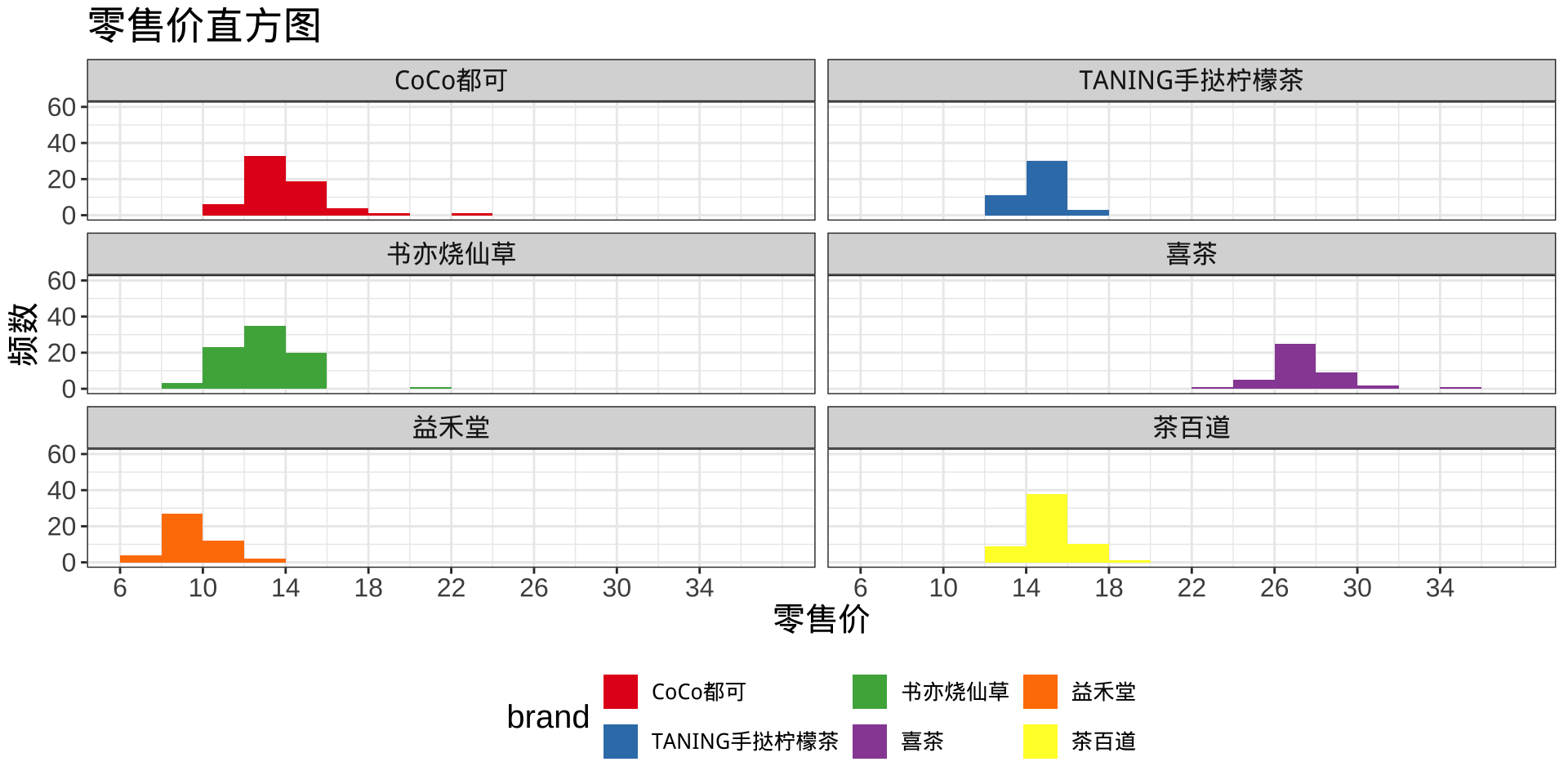

零售价格：喜茶>茶百道>TANNING>CoCo都可>书亦烧仙草>益禾堂

2.4 分组箱线图

data %>% 
  ggplot(aes(retail.price, reorder(brand, retail.price, FUN = median),
             col = brand))+
  geom_boxplot()+
  labs(title ="六大奶茶品牌零售价格",
       x = "零售价格",
       y = "品牌", fill = "品牌")+
  theme_bw() +
  theme(text = element_text(size = 15),
        legend.position = "bottom",
        legend.text = element_text(size = 10))

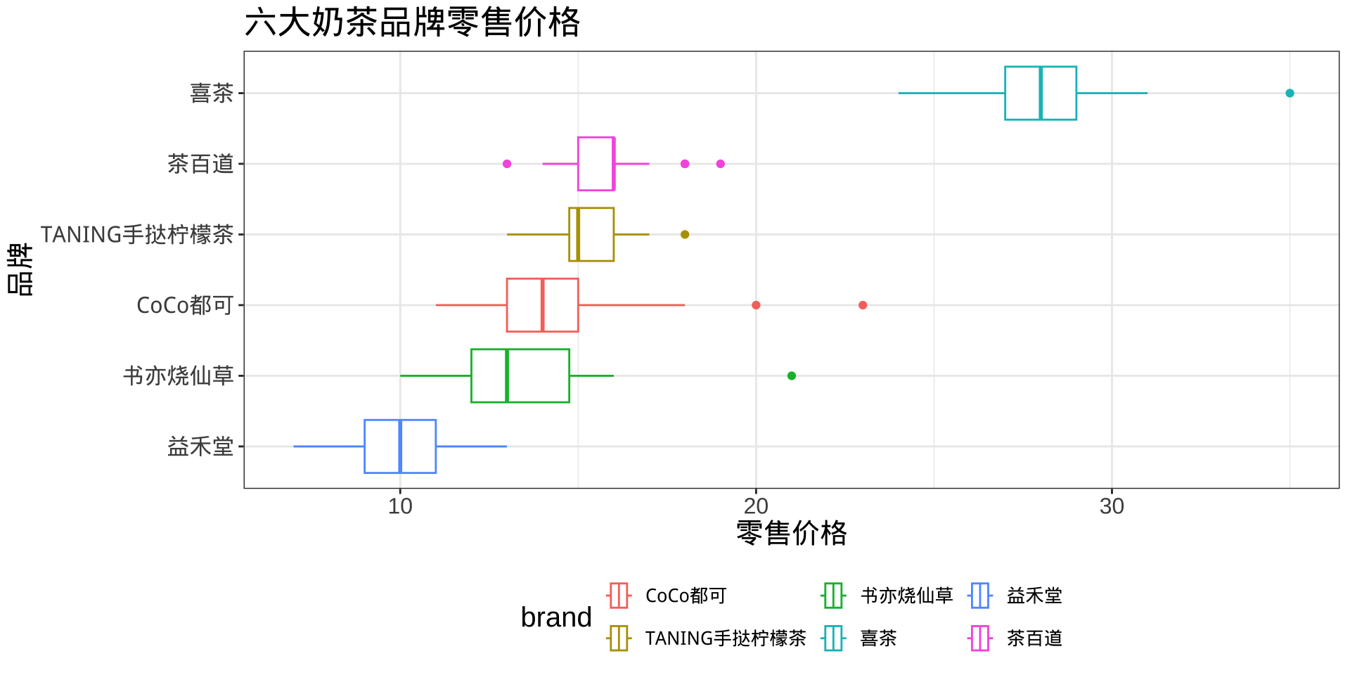
零售价格：喜茶>茶百道>TANNING>CoCo都可>书亦烧仙草>益禾堂

2.5 散点图

data %>% 
  ggplot(aes(retail.price, groupbuy.price,col = brand))+
  geom_point()+
  geom_jitter()+
  geom_smooth(method = lm, se = F) +
  labs(title = "零售价格与团购价散点图",
       x = "零售价",
       y = "团购价") +
  theme_bw() +
    theme(text = element_text(size = 15),
        legend.position = "bottom",
        legend.text = element_text(size = 10))

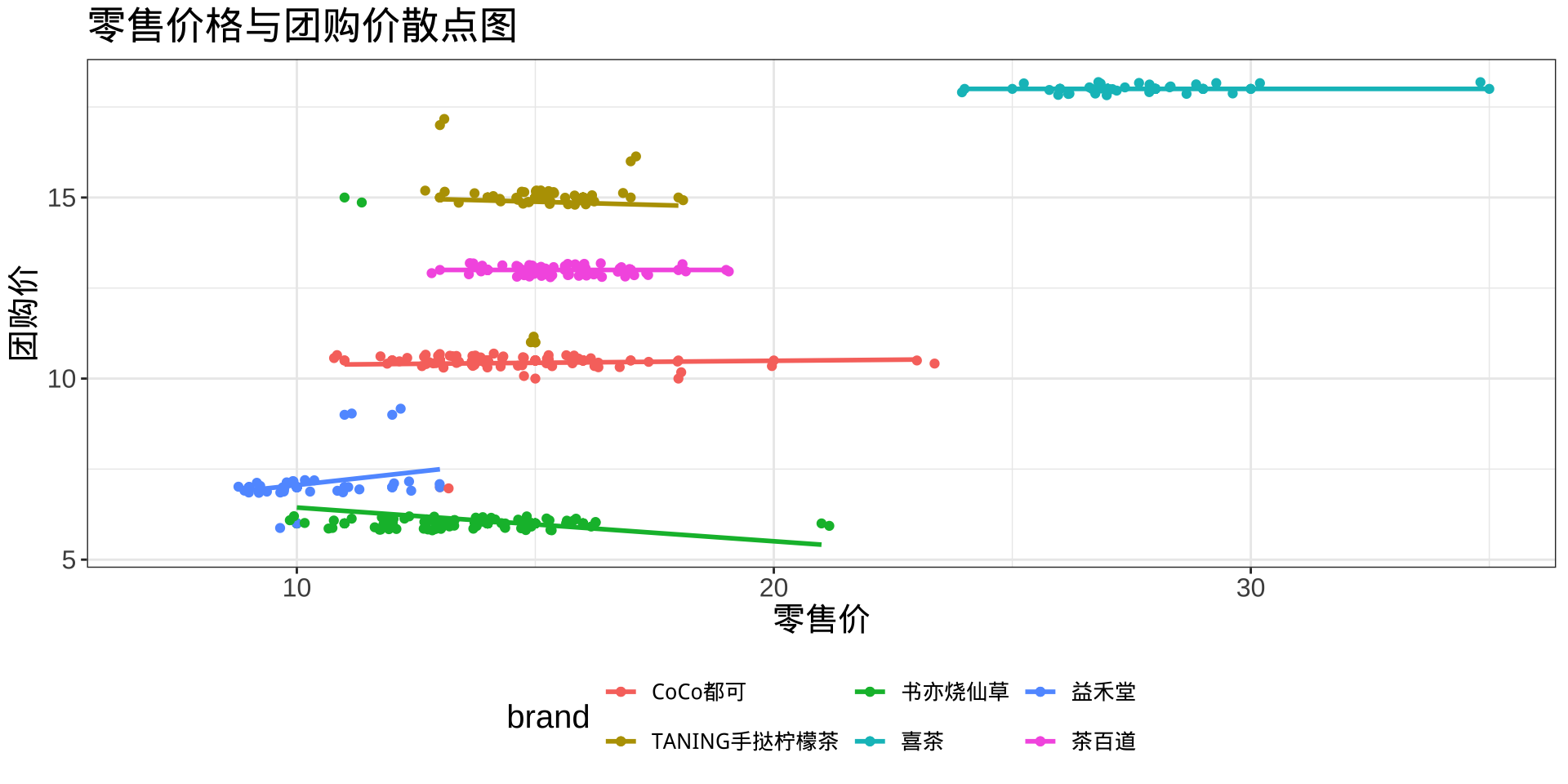
无论在市区、近郊、远郊，同一品牌的团购价格相同。

3 报告描述性统计量

全样本

分品牌零售价格比较

分区域零售价格比价

3.1 全样本

library(psych)

data %>% 
  select(retail.price, groupbuy.price, comment.num) %>%
  describe() %>% 
  select(n, mean, sd, median, min, max, skew, kurtosis)

                 n   mean      sd median min   max skew kurtosis
retail.price   336  15.60    5.26   15.0   7    35 1.53     1.72
groupbuy.price 301  10.85    4.00   10.5   6    18 0.22    -1.15
comment.num    336 564.28 1027.57  281.0  13 10598 5.24    36.47

表格中添加分布图像

{gtExtras}

library(gtExtras)

data %>% 
  select(retail.price, groupbuy.price) %>%
  gt_plt_summary()

.
336 rows x 2 cols
	Column	Plot Overview	Missing	Mean	Median	SD
	retail.price		0.0%	15.6	15.0	5.3
	groupbuy.price		10.4%	10.9	10.5	4.0

表格中添加分布图像

{gtExtras}

retail_group <- data %>% 
  select(brand, retail.price) %>%
  group_by(brand) %>%
  summarize(mean = mean(retail.price) %>% round(3),
            median = median(retail.price)%>% round(3),
            sd = sd(retail.price)%>% round(3),
            retail_t = list(retail.price))


retail_group %>%
  arrange(desc(mean)) %>% 
  gt() %>% 
  gt_plt_dist(retail_t,
              type = "histogram",
              line_color = "purple",
              fill_color = "green",
              bw = 1)

brand	mean	median	sd	retail_t
喜茶	27.930	28	1.818
茶百道	15.603	16	1.154
TANING手挞柠檬茶	15.023	15	1.067
CoCo都可	14.391	14	2.013
书亦烧仙草	13.415	13	1.770
益禾堂	10.067	10	1.286

3.2 分品牌零售价格比较

data %>%
  group_by(brand) %>%
  summarize(n(),
            min = min(retail.price),
            q1 = quantile(retail.price, 0.25),
            median = median(retail.price),
            mean = mean(retail.price),
            q3 = quantile(retail.price, 0.75),
            max = max(retail.price),
            sd = sd(retail.price)) %>% 
  arrange(desc(median))

# A tibble: 6 × 9
  brand            `n()`   min    q1 median  mean    q3   max    sd
  <chr>            <int> <dbl> <dbl>  <dbl> <dbl> <dbl> <dbl> <dbl>
1 喜茶                43    24  27       28  27.9  29      35  1.82
2 茶百道              58    13  15       16  15.6  16      19  1.15
3 TANING手挞柠檬茶    44    13  14.8     15  15.0  16      18  1.07
4 CoCo都可            64    11  13       14  14.4  15      23  2.01
5 书亦烧仙草          82    10  12       13  13.4  14.8    21  1.77
6 益禾堂              45     7   9       10  10.1  11      13  1.29

零售价格：喜茶>茶百道>TANNING>CoCo都可>书亦烧仙草>益禾堂

3.3 分区域零售价格比较

library(psych)

data %>%
  group_by(area) %>%
  summarize(n(),
            min = min(retail.price),
            q1 = quantile(retail.price, 0.25),
            median = median(retail.price),
            mean = mean(retail.price),
            q3 = quantile(retail.price, 0.75),
            max = max(retail.price),
            sd = sd(retail.price))%>% 
  arrange(desc(median))

# A tibble: 3 × 9
  area  `n()`   min    q1 median  mean    q3   max    sd
  <chr> <int> <dbl> <dbl>  <dbl> <dbl> <dbl> <dbl> <dbl>
1 市区    168     8    13     15  16.5  16.2    35  5.90
2 近郊    138     7    13     14  14.7  16      30  4.20
3 远郊     30     8    11     14  14.5  16      28  5.06

零售价格：市区>近郊>远郊

4 研究结论

• 门店数量：书亦烧仙草>CoCo都可>茶百道>益禾堂>TANNING>喜茶

• 零售价格：喜茶>茶百道>TANNING>CoCo都可>书亦烧仙草>益禾堂

• 团购价格：喜茶>TANNING>茶百道>CoCo都可>益禾堂>书亦烧仙草

• 无论在市区、近郊、远郊，同一个品牌的团购价格相同。

• 零售价格：市区>近郊>远郊

5 经验分享

• 数据来源

• 清洗数据

• R代码

• {gtExtras}

• 提炼结论

Thanks for your attention！