# A tibble: 12 × 4
class drv n percent
<chr> <chr> <int> <dbl>
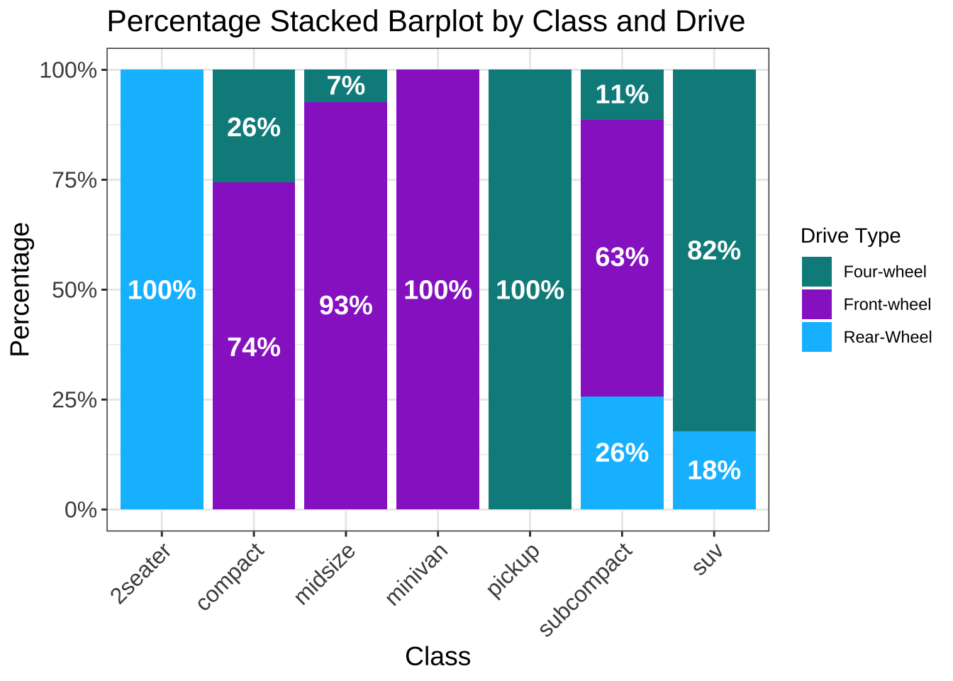
1 2seater r 5 1
2 compact 4 12 0.26
3 compact f 35 0.74
4 midsize 4 3 0.07
5 midsize f 38 0.93
6 minivan f 11 1
7 pickup 4 33 1
8 subcompact 4 4 0.11
9 subcompact f 22 0.63
10 subcompact r 9 0.26
11 suv 4 51 0.82
12 suv r 11 0.18
ggplot(mpg_percent, aes(class, n, fill = drv)) +geom_bar(stat ="identity", position ="fill") +geom_text(aes(label = scales::percent(percent, accuracy =1), y = percent), position =position_fill(vjust =0.5), size =5,fontface ="bold",color ="white") +scale_fill_manual(values =c("cyan4", "darkorchid","deepskyblue"),label =c("Four-wheel","Front-wheel","Rear-Wheel"),name ="Drive Type") +scale_y_continuous(labels = scales::percent_format(accuracy =1))+labs(title ="Percentage Stacked Barplot by Class and Drive", x ="Class", y ="Percentage") +theme(legend.position ="bottom") +theme_bw() +guides(x =guide_axis(angle =45)) +theme(axis.text.x =element_text(size =12), # 设置 x 轴刻度字体大小为 12axis.text.y =element_text(size =12), # 设置 y 轴刻度字体大小为 12axis.title =element_text(size =14), # 设置坐标轴标题字体大小为 14plot.title =element_text(size =16) # 设置图表标题字体大小为 16 )
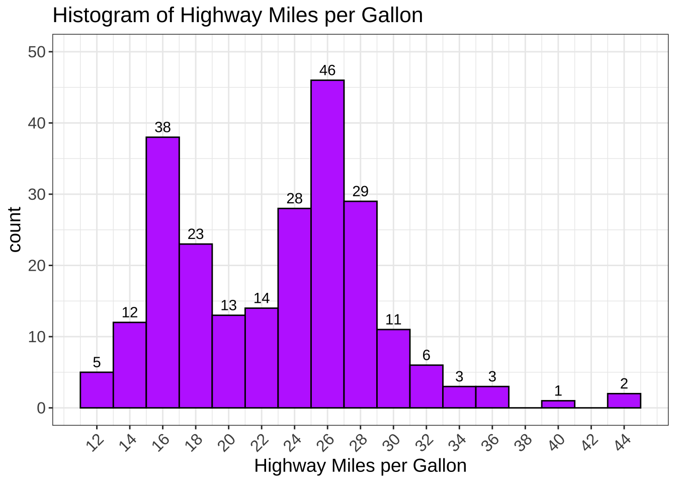
3 直方图频数标注位置不当
summary(mpg$hwy)
   Min. 1st Qu.  Median    Mean 3rd Qu.    Max.
  12.00   18.00   24.00   23.44   27.00   44.00
mpg %>%ggplot(aes(hwy))+geom_histogram(fill ="darkorchid1",color ="black",binwidth =2)+stat_bin(aes(label =ifelse(after_stat(count) ==0,"",after_stat(count))), binwidth =2, geom ="text",vjust =-0.5)+scale_y_continuous(limits =c(0,50), breaks =seq(0,50,10))+scale_x_continuous(breaks =seq(12,44,2))+labs(title ="Histogram of Highway Miles per Gallon",x ="Highway Miles per Gallon") +theme_bw() +guides(x =guide_axis(angle =45)) +theme(axis.text.x =element_text(size =12), # 设置 x 轴刻度字体大小为 12axis.text.y =element_text(size =12), # 设置 y 轴刻度字体大小为 12axis.title =element_text(size =14), # 设置坐标轴标题字体大小为 14plot.title =element_text(size =16) # 设置图表标题字体大小为 16 )
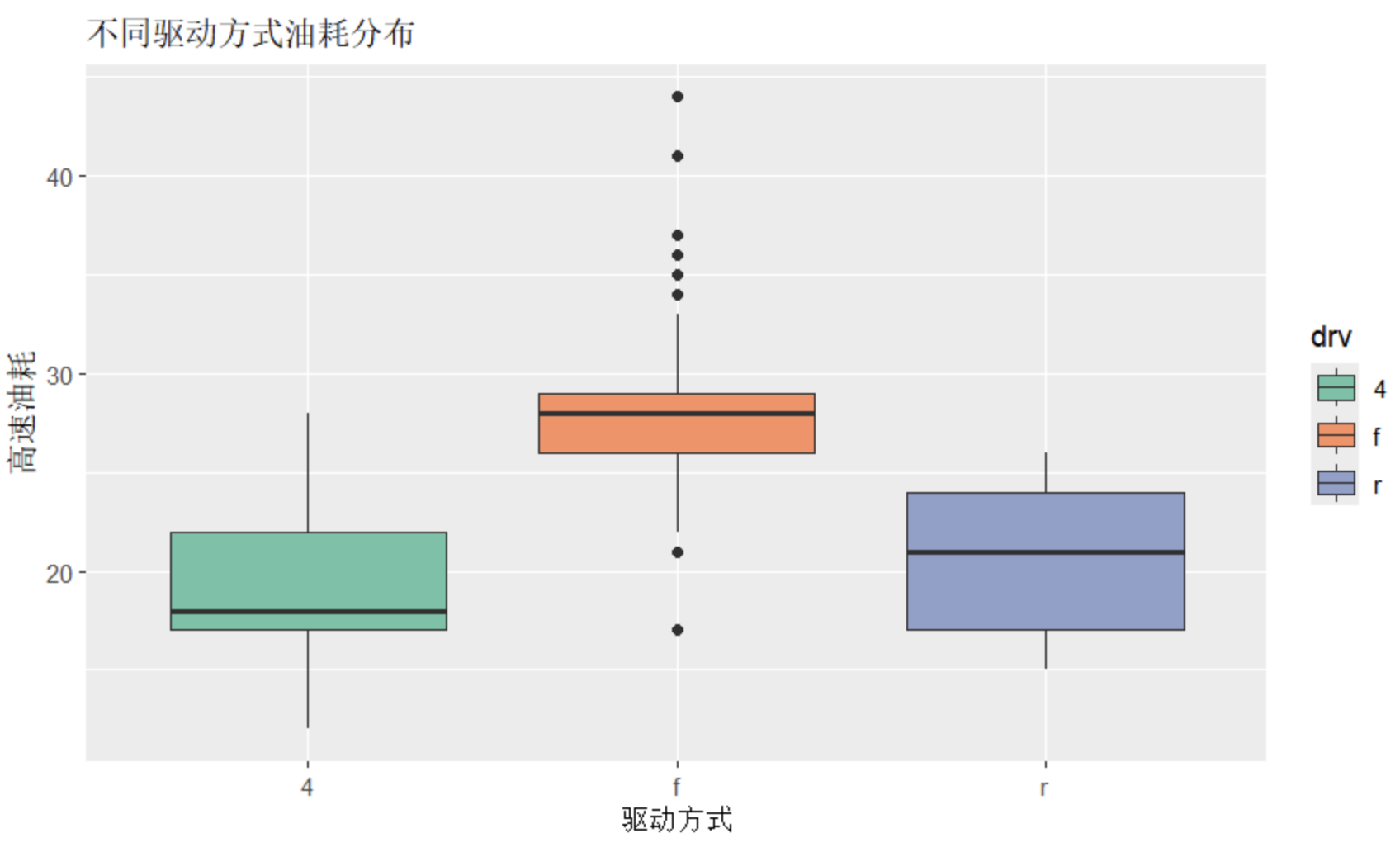
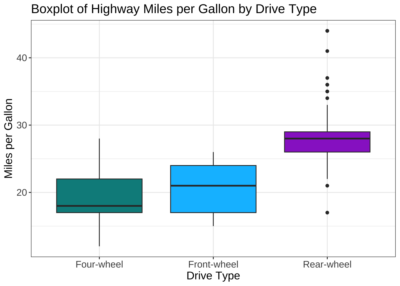
4 箱线图——按定量变量的中位数降序排列
mpg %>%ggplot(aes(fct_reorder(drv, hwy), hwy, fill = drv)) +geom_boxplot() +scale_fill_manual(values =c("cyan4", "darkorchid","deepskyblue")) +scale_x_discrete(labels =c("Four-wheel","Front-wheel","Rear-wheel")) +labs(title ="Boxplot of Highway Miles per Gallon by Drive Type", x ="Drive Type", y ="Miles per Gallon") +theme_bw() +theme(legend.position ="none",axis.text.x =element_text(size =12), # 设置 x 轴刻度字体大小为 12axis.text.y =element_text(size =12), # 设置 y 轴刻度字体大小为 12axis.title =element_text(size =14), # 设置坐标轴标题字体大小为 14plot.title =element_text(size =16) # 设置图表标题字体大小为 16 )
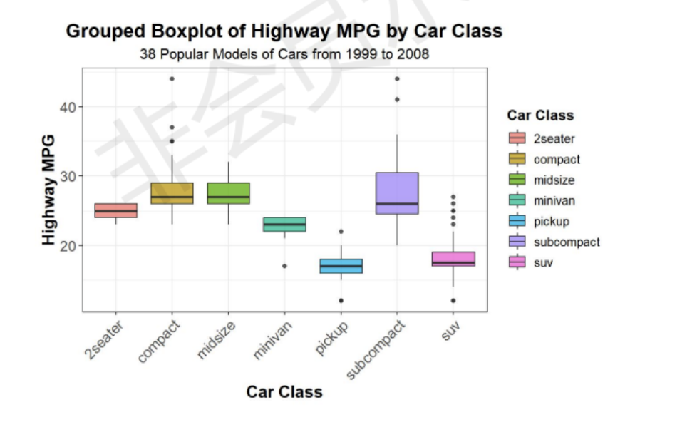
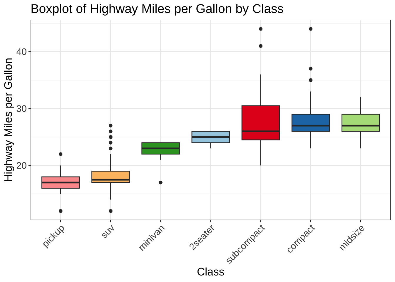
5 箱线图——按定量变量的中位数降序排列
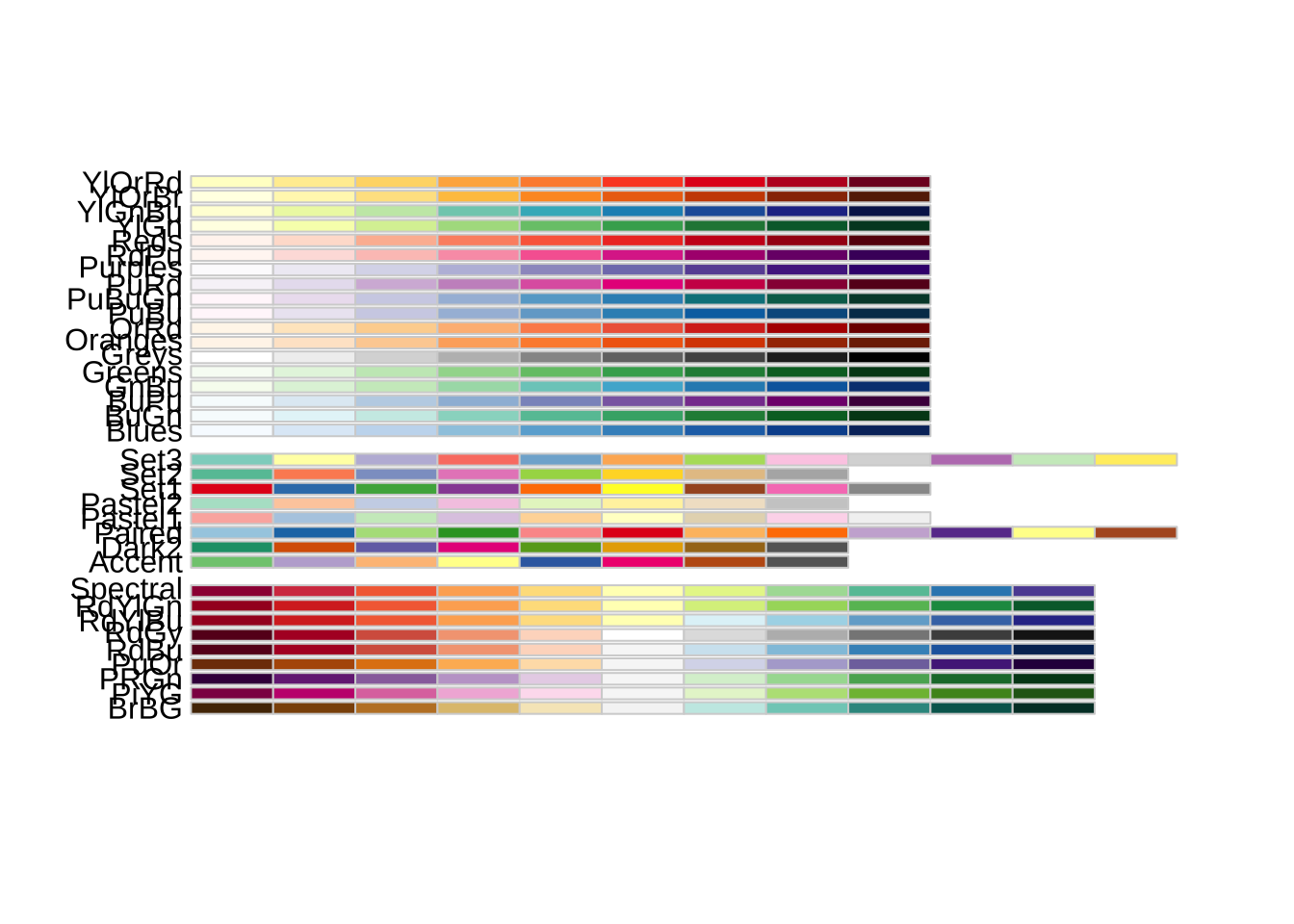
library(RColorBrewer)#查看调色板display.brewer.all()
mpg %>%ggplot(aes(fct_reorder(class, hwy), hwy, fill = class)) +geom_boxplot() +scale_fill_brewer(palette ="Paired")+labs(title ="Boxplot of Highway Miles per Gallon by Class", x ="Class", y ="Highway Miles per Gallon") +theme_bw() +guides(x =guide_axis(angle =45)) +theme(legend.position ="none",axis.text.x =element_text(size =12), # 设置 x 轴刻度字体大小为 12axis.text.y =element_text(size =12), # 设置 y 轴刻度字体大小为 12axis.title =element_text(size =14), # 设置坐标轴标题字体大小为 14plot.title =element_text(size =16) # 设置图表标题字体大小为 16 )
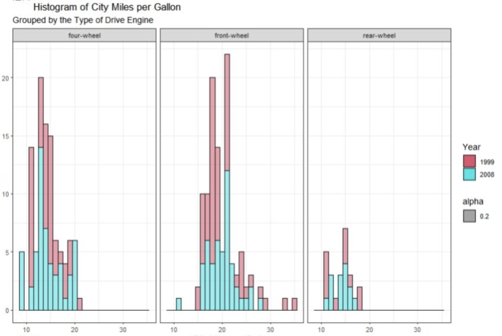
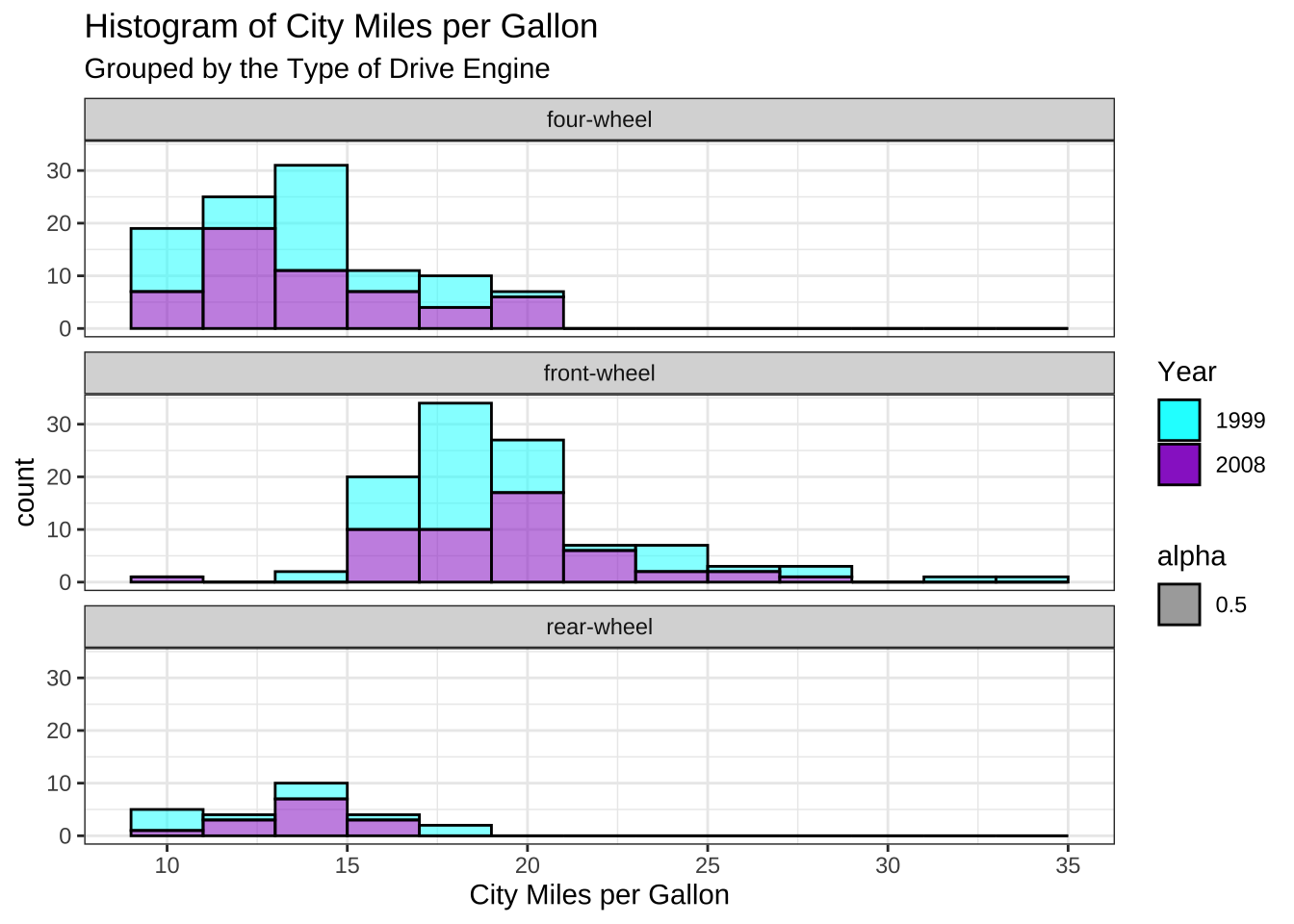
6 图形比例不适当
mpg %>%ggplot(aes(cty, fill =factor(year), # 设置分组变量,factor(year) 将 year数值变量转换为因子变量alpha =0.5))+geom_histogram(binwidth =2, col =1)+facet_wrap(~ drv, # 设置切面变量labeller =labeller(drv =c("4"="four-wheel","f"="front-wheel","r"="rear-wheel")), # 设置切面标签ncol =1)+theme_bw()+scale_fill_manual(values =c("cyan", "darkorchid"))+labs(title ="Histogram of City Miles per Gallon",subtitle ="Grouped by the Type of Drive Engine",x ="City Miles per Gallon",fill ="Year")